OGC Made Easy: Tiling Spec
By: Tim Schaub on May 12 2023
Looking for help getting started with the Open Geospatial Consortium (OGC) API Tiles specification? This primer can get you going.
OGC Made Easy: Tiles
The Open Geospatial Consortium (or OGC) publishes standards related to geospatial information services and formats. The organization recently published “OGC API - Tiles - Part 1: Core” – a specification aimed at web map tile services. The standard weighs in at 137 pages and depends on another 273 page standard, so if you are new to OGC specifications, getting started can be intimidating. The goal of this post is to provide a quickstart for tiled map providers who might want to implement the standard but are struggling to know where to begin.
What’s in a name?
The “OGC API - Tiles - Part 1: Core” specification name is quite a mouthful. The rest of this post will use "OGC Tiles" as a shorthand, but it is worth picking apart the name first.
The previous generation of OGC standards had titles like "Web Map Service" (WMS), "Web Feature Service" (WFS), and "Web Coverage Service" (WCS). These were affectionately referred to as the WxS standards. The "OGC API" prefix in this new specification’s name refers to the new generation of standards designed to work in harmony with existing web standards and best practices – so things like content negotiation and HTTP status codes aren’t redefined by the standards themselves.
The "Tiles" part of the name is what this standard is really about. Before the Google Maps era, maps on web pages were often provided by services that would generate map images of arbitrary places on demand. It is generally faster and more efficient to render map images ahead of time and to cut these images up into regular grids of tiles. The OGC Tiles specification describes how mapping clients (like web pages) can get information about tilesets and how to request the tiled data itself.
The "Part 1: Core" suffix in the standard’s name implies that additional parts will be published in the future describing functionality beyond the core. The core concerns itself with how to provide metadata about a tileset, how to describe the tiling scheme, and how to relate a tileset to a geospatial data collection that might have other representations. The core also discusses how a tileset with a temporal dimension can be handled.
Prior art
For the last 18 years since the launch of Google Maps, people who develop mapping applications on the web have been consolidating on a common scheme for serving tiled map data. The tiles in this scheme fit into a conceptual pyramid where each tile can be identified by three parameters: zoom level (Z), column (X), and row (Y). This has become known as the XYZ tiling scheme.
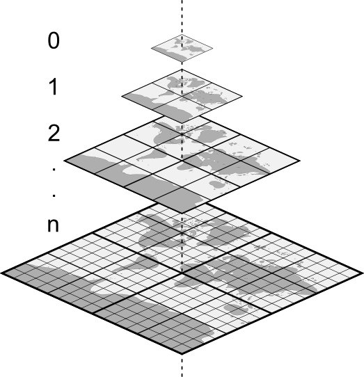
In an XYZ tileset, the 0/0/0 tile at the top usually covers the whole world, and each level below contains four tiles for every one tile above. Most XYZ tilesets use the same Web Mercator projection as Google Maps. XYZ tiles are usually available with a URL that looks like this: https://example.com/tiles/{z}/{x}/{y}.png. In this URL template, {z} is a placeholder for the zoom level, {x} for the column number, and {y} for the row number. The available zoom, column, and row values generally start with zero. The zoom level may extend to something in the 20s for "street level" data.
Of course all of these things (extent, projection, URL template, maximum level) may vary from tileset to tileset. The Mapbox TileJSON specification formalizes how some of this variety can be described in a simple JSON document. One notable constraint of TileJSON is that tilesets must use the Web Mercator projection popularized by Google Maps.
Conformance
The OGC Tiles specification builds on what people have been doing for years with XYZ tilesets and goes beyond what is possible to describe with TileJSON. The standard is organized into conformance classes that build on one another to handle increasingly complex use cases.
The good news is that if you have an existing XYZ tileset, you are (most likely) already OGC Tiles compliant! The Core Conformance Class boils down to three unconditional requirements:
- Tiles must be available using a URL built from a template like
https://example.com/tiles/{z}/{x}/{y}.png(see Requirement 1 for more detail). - Successful responses must have a
200status code (see Requirement 5 for more detail). - Responses for tiles that do not exist must have a
400or404status code (see Requirement 6 for more detail).
The Core Conformance Class in OGC Tiles has additional requirements that only kick in under certain conditions. For example, if you also conform to the Core Conformance Class from the separate “OGC API - Common - Part 1: Core” standard, then requirements 2, 3, and 4 in the Tiles standard say that you have to use {tileMatrix} instead of {z}, {tileRow} instead of {y}, and {tileCol} instead of {x} in your tile URL template (but the core doesn’t have any requirements about how this tile URL template is advertised).
If you have an XYZ tileset and you pass the list of requirements above, then you can say that you implement the Core Conformance Class from the "OGC API - Tiles - Part 1: Core" specification. The OGC Common standard describes a formal way to advertise which conformance classes are implemented. For example, if you conform with the Core Tile requirements and the Core Common requirements, you would advertise this with a document like this:
{
  "conformsTo": [
    "http://www.opengis.net/spec/ogcapi-common-1/1.0/conf/core",
    "http://www.opengis.net/spec/ogcapi-tiles-1/1.0/conf/core"
  ]
}
The Core Conformance Class from the "OGC API - Common - Part 1: Core" standard requires that a conformance document like the one above is available at a /conformance path relative to the root of your service. So a service at https://example.com/ would make the conformance document available at https://example.com/conformance.
Beyond the core
The Core Conformance Class in OGC Tiles adds a bit of formality to what people have already been doing with XYZ tilesets. If you want to provide additional metadata about your tilesets, you can make use of the conformance classes beyond Core. The next set of requirements to consider are part of the Tileset Conformance Class. You might choose to implement these requirements if your tileset doesn’t cover the whole world, if you want to let clients know about a limited set of available zoom levels, or if you use an alternative projection, for example.
The Tileset Conformance Class depends on a separate standard, “OGC Two Dimensional Tile Matrix Set and Tile Set Metadata” (referred to as TMS below), to define the structure of the tileset metadata. Examples are included below, but if all you want is the JSON Schema for tileset metadata, you can find that here: https://schemas.opengis.net/tms/2.0/json/tileSet.json.
Here is an example tileset metadata document that describes the XYZ OpenStreetMap tiles:
{
  "title": "OpenStreetMap",
  "dataType": "map",
  "crs": "http://www.opengis.net/def/crs/EPSG/0/3857",
  "tileMatrixSetURI": "http://www.opengis.net/def/tilematrixset/OGC/1.0/WebMercatorQuad",
  "links": [
    {
      "title": "Tile URL Template",
      "href": "https://tile.openstreetmap.org/{tileMatrix}/{tileCol}/{tileRow}.png",
      "rel": "item",
      "type": "image/png",
      "templated": true
    },
    {
      "title": "Tiling Scheme",
      "href": "https://ogc-tiles.xyz/tileMatrixSets/WebMercatorQuad",
      "rel": "http://www.opengis.net/def/rel/ogc/1.0/tiling-scheme",
      "type": "application/json"
    }
  ]
}
The optional title provides users with an easy way to identify the tileset. You can also provide an optional description with more information. The dataType is a required property. Values can be map (for rendered raster data), vector (for vector tile data), or coverage (for raw raster data). The crs is an identifier (specifically a URI) that indicates which coordinate reference system is used. The tileMatrixSetURI is an identifier for the tiling scheme used. The coordinate reference system and tiling scheme shown corresponds to the setup popularized by Google Maps (zoom level zero has one 256 x 256 pixel tile covering the world in Web Mercator; every level below has four tiles for each tile above). The links property includes a link to the tiling scheme definition (also referred to as tile matrix set). As an alternative to linking to a separate document with the tiling scheme definition, the definition can be included in the tileset metadata using a tileMatrixSet property (this is Requirement 17 of the TMS standard). Finally, and most importantly, the links list includes the tile URL template for requesting individual tiles.
One of the most useful reasons to implement the requirements of the Tileset Conformance Class is to let clients know that a tileset is not available for the whole world. The boundingBox property of the tileset metadata serves this purpose, and including it enables a client to automatically zoom to exactly where there are tiles available. Here is an example bounding box member that indicates that tiles are only available north of the equator and west of the prime meridian (see the tileset-bbox.json for a complete example that includes the whole world as a bounding box):
"boundingBox": {
  "crs": "http://www.opengis.net/def/crs/OGC/1.3/CRS84",
  "lowerLeft": [-180, 0],
  "upperRight": [0, 90]
}
The tileset metadata can also include a tileMatrixSetLimits property. It is recommended that tilesets with limited extent (compared to the extent of the tiling scheme) use this property in addition to the boundingBox to describe those limits.
The tileMatrixSetLimits property is also useful to describe a limited set of zoom levels. For example, if only zoom levels 2 and 3 were available for a particular tileset, the limits could be described with this metadata (see the tileset-limits.json for a complete example):
"tileMatrixSetLimits": [
  {
    "tileMatrix": "2",
    "minTileRow": 0,
    "maxTileRow": 1,
    "minTileCol": 0,
    "maxTileCol": 1
  },
  {
    "tileMatrix": "3",
    "minTileRow": 0,
    "maxTileRow": 3,
    "minTileCol": 0,
    "maxTileCol": 3
  }
]
The above tileMatrixSetLimits only limit the available zoom levels or tile matrix levels. To limit the available extent as well, adjust the minimum and maximum column and row values. The JSON schema for this property is available here: https://schemas.opengis.net/tms/2.0/json/tileMatrixLimits.json.
Next steps
The OGC Tiles standard describes additional sets of requirements beyond the Core and Tileset Conformance Classes. For example, the Tileset List Conformance Class includes requirements for describing a list of tilesets with a subset of the metadata required for an individual tileset (see Requirement 9 and 10). In addition, the OGC Common standard includes requirements that can be useful if your tilesets are related to other geospatial data collections. The OGC API family of standards leverages OpenAPI and JSON Schema for describing services. If your tileset is provided by a service that already makes use of OpenAPI, it can be useful to implement the OpenAPI Conformance Class of the OGC Common standard.
Because these requirements are spread across multiple specifications with slightly different conventions and vocabulary, it can be a challenge to get started if you want to implement a compliant tile service. We put together a go-ogc library and a xyz2ogc utility to help bootstrap the process. You can use the xyz2ogc generate command to produce metadata documents describing an existing XYZ tileset that satisfies the requirements of the conformance classes discussed above. See https://ogc-tiles.xyz/ for a complete set of metadata documents representing some common XYZ tilesets.
Be sure to share your experiences using OGC Tiles with us at https://community.planet.com/developers-55. Follow us on Twitter @PlanetDevs. Sign up for Wavelengths, the Planet Developer Relations newsletter, to learn more about our workflows and get announcements about what is new.
Lightweight GIS pipelines with fio-planet
By: Sean Gillies on April 27 2023
Planet’s new CLI has no builtin GIS capabilities other than what Planet’s APIs provide. To help make more sophisticated workflows possible, Planet is releasing a new package of command line programs for manipulating streams of GeoJSON features.
Making Command Line GIS Pipelines with fio-planet
Planet’s new command line interface (CLI) has no builtin GIS capabilities other than what Planet’s APIs provide. This is by design; it is meant to be complemented by other tools. To help make more sophisticated workflows possible, Planet is releasing a new package of command line programs, fio-planet, which let you build Unix pipelines for manipulating streams of GeoJSON features. Feature simplification before searching the Data API is one such application.
Planet’s new command line interface (CLI) has three main jobs. One is to help you prepare API requests. Planet’s APIs and data products have many options. The CLI provides tools to make specifying what you want easy. Another purpose is to make the status of those requests visible. Some requests take a few minutes to be fulfilled. The CLI permits notification when they are done, like the following command line output.
planet orders wait 65df4eb0-e416-4243-a4d2-38afcf382c30 && cowsay "your order is ready for download"
__________________________________
< your order is ready for download >
 ----------------------------------
        \   ^__^
         \  (oo)\_______
            (__)\       )\/\
                ||----w |
                ||     ||
Or you may prefer to leave cows alone and just download the order when it is ready.
planet orders wait 65df4eb0-e416-4243-a4d2-38afcf382c30 && planet orders download 65df4eb0-e416-4243-a4d2-38afcf382c30
The third purpose of the CLI is to print API responses in a form that lets them be used as inputs to other CLI programs such as jq, the streaming JSON filter. CLI commands, generally speaking, print newline-delimited streams of JSON objects or GeoJSON features.
By design, the CLI has limited options for manipulating JSON and relies heavily on jq. The CLI docs have many examples of usage in combination with jq. Similarly, the CLI outsources GIS capabilities to other programs. One option is the inscrutable and venerable ogr2ogr, but it is not as handy with streaming JSON or GeoJSON as jq is.
To help make sophisticated command line geo-processing workflows more accessible, Planet is releasing a package of command line programs that let you build Unix pipelines for manipulating streams of GeoJSON features. Feature simplification before searching the Data API is one of the many applications.
Processing GeoJSON with fio and fio-planet
The Python package Fiona includes a CLI designed around streams of GeoJSON features. The fio-cat command streams GeoJSON features out of one or more vector datasets. The fio-load command performs the reverse operation, streaming features into GIS file formats. Two Shapefiles with the same schema can be combined into a GeoPackage file using the Unix pipeline below.
fio cat example1.shp example2.shp | fio load -f GPKG examples.gpkg
Note: pipeline examples in this blog post assume a POSIX shell such as bash or zsh. The vertical bar | is a “pipe”. It creates two processes and connects the standard output stream of one to the standard input stream of the other. GeoJSON features pass through this pipe from one program to the other.
Planet’s new fio-planet package fits into this conceptual framework and adds three commands to the fio toolbox: fio-filter, fio-map, and fio-reduce. These commands provide some of the features of spatial SQL, but act on features in a GeoJSON feature sequence instead of rows in a spatial table. Each command accepts a JSON sequence as input, evaluates an expression in the context of the sequence, and produces a new JSON sequence as output. These may be GeoJSON sequences.
- fio-filter evaluates an expression for each feature in a stream of GeoJSON features, passing those for which the expression is true.
- fio-map maps an expression over a stream of GeoJSON features, producing a stream of new features or other values
- fio-reduce applies an expression to a sequence of GeoJSON features, reducing them to a single feature or other value.
In combination, many transformations are possible with these three commands.
Expressions take the form of parenthesized, comma-less lists which may contain other expressions. The first item in a list is the name of a function or method, or an expression that evaluates to a function. It’s a kind of prefix, or Polish notation. The second item is the function's first argument or the object to which the method is bound. The remaining list items are the positional and keyword arguments for the named function or method. The list of functions and callables available in an expression includes:
- Python builtins such as dict, list, and map
- From functools: reduce
- All public functions from itertools, for example, islice, and repeat
- All functions importable from Shapely 2.0, for example, Point, and unary_union
- All methods of Shapely geometry classes
Let’s look at some examples. Below is an expression that evaluates to a Shapely Point instance. Point is a callable instance constructor and the pair of 0 values are positional arguments. Note that the outermost parentheses of an expression are optional.
(Point 0 0)
Fio-planet translates that to the following Python expression.
from shapely import Point
Point(0, 0)
Next is an expression which evaluates to a Polygon, using Shapely’s buffer function. The distance parameter is computed from its own expression, demonstrating prefix notation once again.
(buffer (Point 0 0) :distance (/ 5 2))
The equivalent in Python is
from shapely import buffer
buffer(Point(0, 0), distance=5 / 2)
Fio-filter and fio-map evaluate expressions in the context of a GeoJSON feature and its geometry attribute. These are named f and g. For example, here is an expression that tests whether the distance from the input feature to the point at 0 degrees North and 0 degrees E is less than or equal to one kilometer (1,000 meters).
(<= (distance g (Point 0 0)) 1000)
fio-reduce evaluates expressions in the context of the sequence of all input geometries, which is named c. For example, the expression below dissolves all input geometries using Shapely's unary_union function.
(unary_union c)
Fio-filter evaluates expressions to true or false. Fio-map and fio-reduce will attempt to wrap expression results as GeoJSON feature objects unless raw results are specified. For more information about expressions and usage, please see the fio-planet project page.
Why does fio-planet use Lisp-like expressions for code that is ultimately executed by a Python interpreter? Fio-planet expressions are intended to allow a small subset of what you can do in GeoPandas, PostGIS, QGIS, or a bespoke Python program. By design, fio-planet’s expressions should help discriminate between workflows that can execute effectively on the command line using GeoJSON and workflows that are better executed in a more powerful environment. A domain-specific language (DSL), instead of a general purpose language, is intended to clarify the situation. Fio-planet’s DSL doesn’t afford variable assignment or flow control, for example. That’s supposed to be a signal of its limits. As soon as you feel fio-planet expressions are holding you back, you are right. Use something else!
The program ogr2ogr uses a dialect of SQL as its DSL. The QGIS expression language is also akin to a subset of SQL. Those programs tend to see features as rows of a table. Fio-planet works with streams, not tables, and so a distinctly different kind of DSL seemed appropriate. It adopted the Lisp-like expression language of Rasterio. Parenthesized lists are very easy to parse and Lisp has a long history of use in DSLs. Hylang is worth a look if you’re curious about a more fully featured Lisp for the Python runtime.
Simplifying shapes with fio-map and fio-reduce
Previously, the Planet Developers Blog published a deep dive into simplifying areas of interest for use with the Planet platform. The takeaway from that post is that it’s a good idea to simplify areas of interest as much as you can. Fio-planet brings methods for simplifying shapes and measuring the complexity of shapes to the command line alongside Planet’s CLI. Examples of using them in the context of the previous post are shown below. All the examples use a 25-feature shapefile. You can get it from rmnp.zip or access it in a streaming fashion as shown in the examples below.
Note: all examples assume a POSIX shell such as bash or zsh. Some use the program named jq. The vertical bar | is a “pipe”. It creates two processes and connects the standard output stream of one to the standard input stream of the other. The backward slash \ permits line continuation and allows pipelines to be typed in a more readable form.
A figure accompanies each example. The figures are rendered from a GeoJSON file by QGIS. The GeoJSON files are made by collecting, with fio-collect, the non-raw output of fio-cat, fio-map, or fio-reduce. For example, the pipeline below converts the zipped Shapefile on the web to a GeoJSON file on your computer.
fio cat zip+https://github.com/planetlabs/fio-planet/files/10045442/rmnp.zip \
| fio collect > rmnp.geojson
Counting vertices in a feature collection
The vertex_count function, in conjunction with fio-map's --raw option, prints out the number of vertices in each feature. The default for fio-map is to wrap the result of every evaluated expression in a GeoJSON feature; --raw disables this. The program jq provides a nice way of summing the resulting sequence of numbers. jq -s “slurps” a stream of JSON objects into an array.
The following pipeline prints the number 28,915.
Input:
fio cat zip+https://github.com/planetlabs/fio-planet/files/10045442/rmnp.zip \
| fio map 'vertex_count g' --raw \
| jq -s 'add'
Output:
28915

Counting vertices after making a simplified buffer
One traditional way of simplifying an area of interest is to buffer it by some distance and then simplify it by a comparable distance. The effectiveness of this method depends on the nature of the data, especially the distance between vertices around the boundary of the area. There's no need to use jq in the following pipeline because fio-reduce prints out a sequence of exactly one value.
Input:
fio cat zip+https://github.com/planetlabs/fio-planet/files/10045442/rmnp.zip \
| fio reduce 'unary_union c' \
| fio map 'simplify (buffer g 40) 40' \
| fio map 'vertex_count g' --raw
Output:
469
Variable assignment and flow control are not provided by fio-planet’s expression language. It is the pipes between commands which afford some assignment and logic. For example, the pipeline above is practically equivalent to the following Python program.
import fiona
from fiona.transform import transform_geom
from shapely import buffer, shape, simplify, mapping, unary_union


with fiona.open("zip+https://github.com/planetlabs/fio-planet/files/10045442/rmnp.zip") as dataset:
    c = [shape(feat.geometry) for feat in dataset]


g = unary_union(c)


g = shape(transform_geom("OGC:CRS84", "EPSG:6933", mapping(g)))
g = simplify(buffer(g, 40), 40)
g = shape(transform_geom("EPSG:6933", "OGC:CRS84", mapping(g)))


print(vertex_count(g))

Counting vertices after merging convex hulls of features
Convex hulls are an easy means of simplification. There are no distance parameters to tweak as there were in the example above. The --dump-parts option of fio-map turns the parts of multi-part features into separate single-part features. This is one of the ways in which fio-map can multiply its inputs, printing out more features than it receives.
The following pipeline prints the number 157.
Input:
fio cat zip+https://github.com/planetlabs/fio-planet/files/10045442/rmnp.zip \
| fio map 'convex_hull g' --dump-parts \
| fio reduce 'unary_union c' \
| fio map 'vertex_count g' --raw
Output:
157

Counting vertices after merging the concave hulls of features
Convex hulls simplify, but also dilate concave areas of interest. They fill the "bays", so to speak, and this can be undesirable. Concave hulls do a better job at preserving the concave nature of a shape and result in a smaller increase of area.
The following pipeline prints the number 301.
Input:
fio cat zip+https://github.com/planetlabs/fio-planet/files/10045442/rmnp.zip \
| fio map 'concave_hull g 0.4' --dump-parts \
| fio reduce 'unary_union c' \
| fio map 'vertex_count g' --raw
Output:
301

Using fio-planet with the Planet CLI
Now for more specific examples of using fio-planet with Planet’s CLI on the command line. If you want to spatially constrain a search for assets in Planet’s catalog or clip an order to an area of interest, you will need a GeoJSON object. The pipeline below creates one based on the data used above and saves it to a file. Note that the fourth piece of the pipeline forces the output GeoJSON to be two-dimensional. Planet’s Data API doesn’t accept GeoJSON with Z coordinates.
fio cat zip+https://github.com/planetlabs/fio-planet/files/10045442/rmnp.zip \
| fio map 'concave_hull g 0.4' --dump-parts \
| fio reduce 'unary_union c' \
| fio map 'force_2d g' \
| fio collect \
> rmnp.geojson
Incorporating that GeoJSON object into a Data API search filter is the next step. The filter produced by the command shown below will find items acquired after Feb 14, 2023 that intersect with the shape of Rocky Mountain National Park.
planet data filter \
--date-range acquired gt 2023-02-14 \
--date-range acquired lt 2023-02-25 \
--geom=rmnp.geojson \
> filter.json
With a filter document, stored here in filter.json – the name of the filter doesn’t matter – you can make a filtered search and stream the GeoJSON results into a file. It’s a common practice to use .geojsons, plural, as the file extension for newline-delimited sequences of GeoJSON features.
planet data search PSScene --filter=filter.json > results.geojsons
The fio-planet commands are useful for processing search results, too. The results.geojsons file contains a stream of GeoJSON features which represent some PSScene items in Planet’s catalog. Here’s an example of finding the eight scenes that cover 40.255 degrees North and 105.615 degrees West (the summit of Longs Peak in Rocky Mountain National Park).
Input:
cat results.geojsons \
| fio filter 'contains g (Point -105.615 40.255)' \
| jq '.id'
Output:
"20230222_172633_18_247f"
"20230221_165059_39_241b"
"20230221_165057_22_241b"
"20230220_171805_27_2251"
"20230219_172658_28_2461"
"20230217_172940_13_2474"
"20230216_171328_72_2262"
"20230214_173045_31_2489"
To further filter by the degree to which the ground is visible in each scene – which could also have been specified in the search filter, by the way – we can add a jq step to the pipeline.
cat results.geojsons \
| fio filter 'contains g (Point -105.615 40.255)' \
| jq -c 'select(.properties.visible_percent > 90)' \
| fio collect \
> psscenes.geojson

Fio-filter and fio-map can also be used as checks on the number of vertices and the area of GeoJSON features. Let’s say that you want to keep your areas of interest to 500 vertices or less and no more than 2,000 square kilometers. You can ask fio-map to print true or false or ask fio-filter to screen out features that don’t meet the criteria.
Input:
fio cat rmnp.geojson \
| fio map -r '& (< (vertex_count g) 500) (< (area g) 2000e6)'
Output:
true
Note that the value returned by the builtin area function has units of meters squared. The area of the feature in the rmnp.geojson file is 1,117.4 square kilometers and has 301 vertices.
Creating search geometries on the command line
What if you want to do a quick search that isn’t related to any particular GIS dataset? The new fio-map command can help.
All of Shapely’s geometry type constructors are available in fio-planet expressions and can be used to create new shapes directly on the command line. Remember that fio-map’s --raw/-r option specifies that the outputs of the command will not be wrapped in GeoJSON feature objects, but returned in their natural, raw form. Another fio-map option, --no-input/-n, specifies that the given expression will be mapped over the sequence [None], as with jq --null-input/-n, producing a single output. Together, these options let fio-map produce new GeoJSON data that is not based on any existing data. On the command line you can combine the options as -nr or -rn. If it helps, think of -rn as “right now”.
Input:
fio map -rn '(Point -105.615 40.255)'
Output:
{"type": "Point", "coordinates": [-105.615, 40.255]}
This value can be saved to a file and used with the planet-data-filter program.
fio map -rn '(Point -105.615 40.255)' > search.geojson
planet data filter --geom search.geojson > filter.json
planet data search PSScene --filter filter.json
Or it can be used inline to make a search without saving any intermediate files at all using POSIX command substitution with the $(...) syntax, although nested substitution takes a heavy toll on the readability of commands. Please speak with your tech lead before putting pipelines like the one below into production.
planet data search PSScene --filter="$(planet data filter --geom="$(fio map -rn '(Point -105.615 40.255)')")"
Creating and simplifying GeoJSON features for use with the Planet CLI are two of the applications for fio-planet’s map, filter, and reduce commands. You can surely think of more! Combine them in different ways to create new pipelines suited to your workflows and share your experience with others in Planet’s Developers Community or in the fio-planet discussion forum.
Next Steps
Keep up to date with the fio-planet GitHub repository and the latest project documentation. Chat with us about your experiences and issues using Fiona and fio-planet with Planet data at https://community.planet.com/developers-55. Follow us on Twitter @PlanetDevs. Sign up for Wavelengths, the Planet Developer Relations newsletter, to get more information on the tech behind the workflows.
Planet's Role in Sustaining the Python Geospatial Stack
By: Sean Gillies on March 16 2023
Can Planet data or the Planet platform be used with Python? It can, and not by accident. Planet is working to make it so. This post attempts to explain what the Python Geospatial Stack is and Planet’s role in keeping the stack in good shape so that developers continue to get value from it.
Planet’s customers don’t only use Planet products via commercial or open source desktop GIS or partner platforms. Many of you are integrating Planet’s products and services into custom-built GIS systems, which use the open source Python Geospatial Stack. This post attempts to explain what the Python Geospatial Stack is and Planet’s role in keeping the stack in good shape so that developers like you continue to get value from it. Can Planet data or the Planet platform be used with Python? It can, and not by accident. Planet is working to make it so. You can help, too.
What is the Python Geospatial Stack?
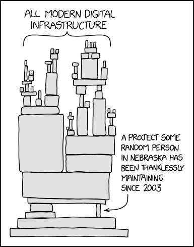
The Python Geospatial Stack is a set of Python packages that use a smaller set of non-standard system libraries written in C/C++: GEOS, PROJ, and GDAL. GEOS is a library of 2-D computational geometry routines. PROJ is a library for cartographic projections and geodetic transformations. GDAL is a model for computing with raster and vector data and a collection of format drivers to allow data access and translation on your computer or over your networks. Planet engineers, including myself, have contributed significantly to these system libraries. Principal Engineer Frank Warmerdam is the author of GDAL, a longtime maintainer of PROJ version 4, and a major contributor to GEOS.
Shapely, Pyproj, Fiona, Rasterio, GeoPandas, PDAL, and Xarray are the core of the stack. Shapely draws upon GEOS. Shapely is useful to developers for filtering asset catalog search results, comparing catalog item footprints to areas of interest, and much more. Pyproj wraps PROJ. Pyproj is helpful for calculating the projected area of regions that are described in longitude and latitude coordinates, and more. Fiona and Rasterio are based on GDAL and allow developers to read and write vector and raster data. PDAL translates and manipulates point cloud data, GeoPandas and Xarray use Fiona and Rasterio and provide higher levels of abstraction for analysis of column-oriented tabular and gridded scalar data, respectively.
How did the stack come about?
Why are so many organizations using Python for GIS work? Isn’t it slow? Only an instructional language? Timing explains a lot. When Bruce Dodson started looking at alternatives to Avenue, the scripting language of Esri's ArcView GIS version 3, Python was ready. Python had a good extension story in 2000, meaning that although Python was relatively slow, it was fairly easy to extend with fast code written in C.
When you compute and dissolve the convex hulls of multiple shapes using Shapely, all of the intensive calculation is done by native code, not Python bytecode. The open source native code (GDAL, GEOS, PROJ, etc) just happened to rise up at the same point in time. Timing really is everything.

To close the loop, the Geospatial Stack has helped make the Python language sticky. Developers chose Python from many options for the availability of solid, feature-rich, decently-documented libraries in a particular domain, and end up staying for all the other nice things about the Python language and community. The reason why Python is the second best language for many domains is that the same discovery happened in Numerical Analysis, Machine Learning, Image Processing, and elsewhere.
How is Planet helping?
Software and software communities need care and feeding. Planet is involved through financial sponsorship, project governance, code maintenance, and builds of binary distributions.
In 2021, Planet became an inaugural platinum sponsor of GDAL. Planet is helping to pay for infrastructure costs and for the labor of full-time maintainers for GDAL and affiliated projects like GEOS and PROJ. In addition, two Planet engineers (Frank Warmerdam and I) serve on GDAL’s project steering committee. The impact of this sponsorship is huge. GDAL has a better and faster build system, which makes it easier to contribute to and which reduces the cost of every bug fix and new feature. Most importantly, the sponsorship makes it possible for GDAL’s longtime maintainers to avoid burnout, stay involved, and mentor their eventual successors.
Planet’s Developer Relations team is mainly involved at the Python level. I’m the release manager for Fiona and Rasterio. I make sure that binary distributions (aka “wheels”) for Linux, MacOS, and Windows are uploaded to Python’s Package Index so that when developers run “pip install rasterio” almost everybody gets pre-compiled Python packages with GDAL, GEOS, and PROJ batteries included. Packages that “just work” for many cases on laptops and in hosted notebooks.
A major new version of Shapely was released at the end of 2022 through collaboration with core GeoPandas developers. Shapely 2.0 adds vectorized operations that radically speed up GeoPandas and keep this piece of the stack relevant as projects like GeoParquet start to change the nature of vector data.
Fiona 1.9.0 was released on Jan 20, 2023 and also provides a boost to GeoPandas. Planet’s Developer Relations team is currently building new tools that integrate with this new version of the Geospatial Stack’s vector data package. They will be announced soon.
Multiple teams at Planet helped make Rasterio 1.3.0, Shapely 2.0.0, and Fiona 1.9.0 successful releases by testing beta releases of these packages. Planet is financially sustaining the open source projects that form the foundation of the stack. The DevRel team is engaged with the open source communities that write the stack’s code. At Planet we consider the health of the Python Geospatial Stack to be a big factor in the overall experience of our platform.
Next Steps
Are you using Fiona, Rasterio, or Shapely? Upgrade to the latest versions and try them out. Chat with us about any ideas or issues with using these packages with Planet data at https://community.planet.com/developers-55. Follow us on twitter @planetdevs.
GEE Integration: a Planet Developers Deep Dive
By: Kevin Lacaille on February 23 2023
Directly Integrating Planet Data Delivery with Google Earth Engine
Do you need some time and space?
With Planet’s high resolution, multi-band, daily imagery, with large color depth, users have a lot of data! Do you find your computer always reminding you that you need to “make more space available?” Are you always running late because your data processing is taking too long? Please let me present:
 |
 |
Google Earth Engine, or GEE for short, is a cloud-based platform for geospatial analysis and remote sensing applications. It is part of Google’s larger Earth platform, which includes the popular Google Earth mapping software. GEE gives users the opportunity to store their Planet data on Google’s cloud storage and harness Google’s computing infrastructure. GEE is used to analyze and monitor the Earth’s changing environment. It can be used to measure land cover and vegetation health, track changes in surface water, monitor wildfires, and measure other impacts of climate change. It can also be used to generate maps, 3D models, and other visualizations. GEE has become a popular platform for geospatial analysis and remote sensing applications, and has been used for a range of projects, from monitoring crop yields in Canada to tracking deforestation in the Amazon.
Planet 𝗑 Google
Google Earth Engine is used to run large-scale geospatial data analysis or to perform a few simple commands on geospatial data. GEE leverages Google’s tools and services, and performs computations at scale with a user-friendly interface. This sort of geospatial working environment makes analyzing your Planet data fast and easy.
Planet users can easily have their data delivered directly to their GEE project thanks to Planet’s Google Earth Engine Delivery Integration - a simpler way for GEE users to incorporate Planet data into their existing workflows and ongoing projects. This integration simplifies the GEE delivery experience by creating a direct connection from Planet's Orders API to GEE, so that you don't have to download then re-upload images or spin up temporary cloud storage when moving imagery to your GEE account.
In this blog post we are going to cover:
- How to prepare your Google Earth Engine account for data delivery via Planet’s Orders API
- How to use Planet’s GEE Delivery Integration service on your GEE project
- A basic and advanced example JSON requests and responses
- A Python example using Planet’s Python SDK, hosted in a Jupyter Notebook
- A Planet CLI example
How to deliver your data to GEE
To deliver data to your GEE project, you must first sign up for an Earth Engine account, create a Cloud Project, enable the Earth Engine API, and grant access to a Google service account.
Set up GEE
Before we get into the coding aspect of it all, we need to set up our GEE project.
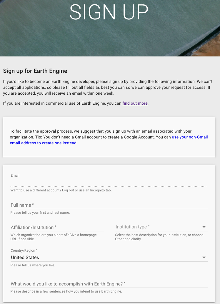
1. Sign up for an EE account
First thing’s first, let’s sign up for an Earth Engine account. Go to: https://signup.earthengine.google.com/
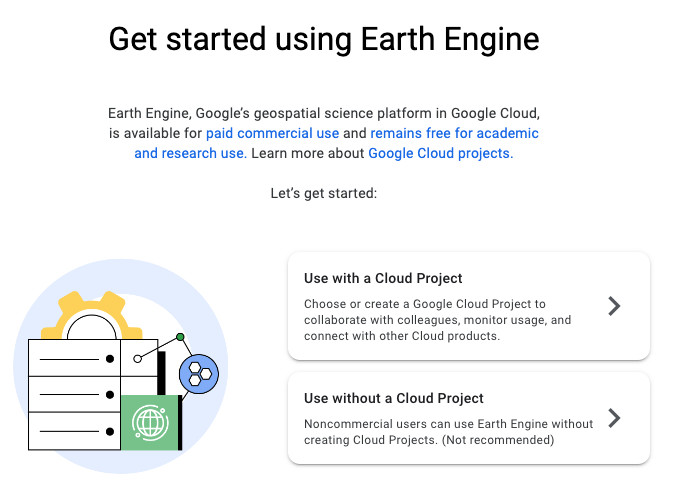
2. Register a Google Cloud Project (GCP) project
Now that you have an Earth Engine account, let’s create a new Cloud Project for your account. This will simultaneously create an empty ImageCollection. This ImageCollection is where all of your data will be delivered to.
Go to: https://code.earthengine.google.com/register/
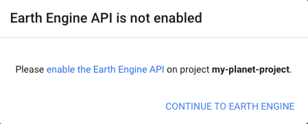
3. Enable the EE API for the project
In order to allow Planet’s Orders API to interact with GEE, we must first enable the Earth Engine API.
Go to: https://console.cloud.google.com/apis/library/earthengine.googleapis.com
4. Grant Planet access to deliver to your GEE project
Lastly, you need to create a service account, which in this case is essentially a virtual account, which will be used to automate our GEE integration. To create this service account, return to the console and select: Navigation menu > IAM & Admin > Service Accounts
Then we can create a service account by clicking “+CREATE SERVICE ACCOUNT”. Here we will add Planet’s Google service account, named planet-gee-uploader@planet-earthengine-staging.iam.gserviceaccount.com
Finally, your service account must be granted the role of “Earth Engine Resource Writer”, which will allow it to deliver your data to your ImageCollection.
Examples
Now that you have a GEE project that Planet has access to, here’s how you tell Planet how to access that GEE project.
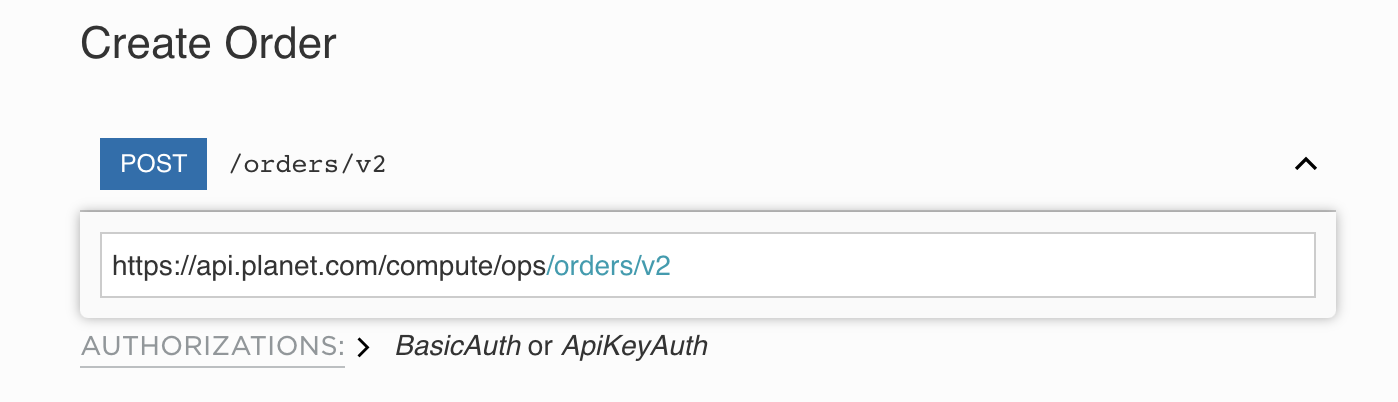
To communicate with Planet’s servers, we use RESTful endpoints. Regardless of the language you use to make a network request, here’s the body of the request. In the language that you use, you’ll need to provide the following to successfully make a request:
- API endpoint (https://api.planet.com/compute/ops/orders/v2)
- Basic auth using your Planet API key
- Header to specify that the
Content-Typeisapplication/json - Body, the specifics of what you’re requesting
Basic JSON request
REST method:
POST https://api.planet.com/compute/ops/orders/v2/
An example JSON request body for delivery for:
- Order name: iowa_order
- Item IDs: 20200925_161029_69_2223, 20200925_161027_48_2223
- Item type: PSScene
- Product bundle: analytic_sr_udm2
- GEE project name: planet-devrel-dev
- ImageCollection name: gee-integration-testing
Request:
{
  "name": "iowa_order",
  "products": [
    {
      "item_ids": [
        "20200925_161029_69_2223",
        "20200925_161027_48_2223"
      ],
      "item_type": "PSScene",
      "product_bundle": "analytic_sr_udm2"
    }
  ],
  "delivery": {
    "google_earth_engine": {
      "project": "planet-devrel-dev",
      "collection": "gee-integration-testing"
    }
  }
}
Response:
{
"_links": {
"_self": "https://api.planet.com/compute/ops/orders/v2/1e4ade86-20dd-45bc-a3cf-4e6f378b5774"
},
"created_on": "2022-11-30T19:08:34.193Z",
"error_hints": [],
"id": "1e4ade86-20dd-45bc-a3cf-4e6f378b5774",
"last_message": "Preparing order",
"last_modified": "2022-11-30T19:08:34.193Z",
"metadata": {
"stac": {}
},
"name": "iowa_order",
"products": [
{
"item_ids": [
"20200925_161029_69_2223",
"20200925_161027_48_2223"
],
"item_type": "PSScene",
"product_bundle": "analytic_sr_udm2"
}
],
"state": "queued"
}
Advanced JSON request
GEE integration also supports two tools, clipping, and sensor harmonization. To include them, we add them to the “tools” schema. Adding to the previous example, if we want to clip to an AOI defined as a polygon and harmonize our data to Sentinel-2’s sensor, the JSON request would look like:
Request:
{
  "name": "iowa_order",
  "products": [
    {
      "item_ids": [
        "20200925_161029_69_2223",
        "20200925_161027_48_2223"
      ],
      "item_type": "PSScene",
      "product_bundle": "analytic_sr_udm2"
    }
  ],
  "delivery": {
    "google_earth_engine": {
      "project": "planet-devrel-dev",
      "collection": "gee-integration-testing"
    }
  },
  "tools": [
    {
      "clip": {
        "aoi": {
          "type": "Polygon",
          "coordinates": [
            [
              [-91.198465, 42.893071],
              [-91.121931, 42.893071],
              [-91.121931, 42.946205],
              [-91.198465, 42.946205],
              [-91.198465, 42.893071]
            ]
          ]
        }
      }
    },
    {
      "harmonize": {
        "target_sensor": "Sentinel-2"
      }
    }
  ]
}
Response:
{
"_links": {
"_self": "https://api.planet.com/compute/ops/orders/v2/1e4ade86-20dd-45bc-a3cf-4e6f378b5774"
},
"created_on": "2022-11-30T19:08:34.193Z",
"error_hints": [],
"id": "1e4ade86-20dd-45bc-a3cf-4e6f378b5774",
"last_message": "Preparing order",
"last_modified": "2022-11-30T19:08:34.193Z",
"metadata": {
"stac": {}
},
"name": "iowa_order",
"products": [
{
"item_ids": [
"20200925_161029_69_2223",
"20200925_161027_48_2223"
],
"item_type": "PSScene",
"product_bundle": "analytic_sr_udm2"
}
],
"state": "queued",
"tools": [
{
"clip": {
"aoi": {
"coordinates": [
[
[-91.198465, 42.893071],
[-91.121931, 42.893071],
[-91.121931, 42.946205],
[-91.198465, 42.946205],
[-91.198465, 42.893071]
]
],
"type": "Polygon"
}
}
},
{
"harmonize": {
"target_sensor": "Sentinel-2"
}
}
]
}
Integration with Python
Users can integrate their Planet data delivery with GEE with Python via Planet’s Python SDK 2.0. Using the SDK, users can generate their request, order data using the Orders API, then have it delivered directly to GEE. For an in-depth example, please see this Jupyter Notebook.
import planet
import asyncio

# The area of interest (AOI) defined as a polygon
iowa_aoi = {
    "type":
    "Polygon",
    "coordinates": [[[-91.198465, 42.893071], [-91.121931, 42.893071],
                     [-91.121931, 42.946205], [-91.198465, 42.946205],
                     [-91.198465, 42.893071]]]
}

# The item IDs we wish to order
iowa_images = ['20200925_161029_69_2223', '20200925_161027_48_2223']
# Google Earth Engine configuration
cloud_config = planet.order_request.google_earth_engine(
    project='planet-devrel-dev', collection='gee-integration-testing')
# Order delivery configuration
delivery_config = planet.order_request.delivery(cloud_config=cloud_config)
# Product description for the order request
data_products = [
    planet.order_request.product(item_ids=iowa_images,
                                 product_bundle='analytic_sr_udm2',
                                 item_type='PSScene')
]

# Build the order request
iowa_order = planet.order_request.build_request(name='iowa_order',
                                                products=data_products,
                                                delivery=delivery_config)

# Create a function to create and deliver an order
async def create_and_deliver_order(order_request, client):
    '''Create and deliver an order.

    Parameters:
        order_request: An order request
        client: An Order client object
    '''
    with planet.reporting.StateBar(state='creating') as reporter:
        # Place an order to the Orders API
        order = await client.create_order(order_request)
        reporter.update(state='created', order_id=order['id'])
        # Wait while the order is being completed
        await client.wait(order['id'],
                          callback=reporter.update_state,
                          max_attempts=0)

    # Grab the details of the orders
    order_details = await client.get_order(order_id=order['id'])

    return order_details

# Create a function to run the create_and_deliver_order function
async def main():
    async with planet.Session() as ps:
        # The Orders API client
        client = ps.client('orders')
        # Create the order and deliver it to GEE
        order_details = await create_and_deliver_order(iowa_order, client)
        return order_details

# Deliver data to GEE and return the order’s details
order_details = asyncio.run(main())
Using the Planet CLI
Lastly, we can use the Planet command line interface (CLI) to deliver data to GEE. If we want to clip or harmonize our data, first we need to create a file called tools.json containing the following information:
[
  {
    "clip": {
      "aoi": {
        "type": "Polygon",
        "coordinates": [
          [
            [-91.198465, 42.893071],
            [-91.121931, 42.893071],
            [-91.121931, 42.946205],
            [-91.198465, 42.946205],
            [-91.198465, 42.893071]
          ]
        ]
      }
    }
  },
  {
    "harmonize": {
      "target_sensor": "Sentinel-2"
    }
  }
]
Then, to order and deliver data with the Planet CLI, we query the Orders API with 3 commands:
1. Generate an order request
The request function requires that you give it an item type, product bundle, an order name, and item IDs.
$ planet orders request \
20200925_161029_69_2223,20200925_161027_48_2223 \
--item-type psscene \
--bundle analytic_sr_udm2 \
--name "iowa_order" \
--tools tools.json \
> my_order.json
Here, we are saving the order request into a file called my_order.json, which we will use to create the order.
2. Create an order
$ planet orders create my_order.json

{"_links": {"_self": "https://api.planet.com/compute/ops/orders/v2/1e4ade86-20dd-45bc-a3cf-4e6f378b5774"}, "created_on": "2022-11-30T19:08:34.193Z", "error_hints": [], "id": "1e4ade86-20dd-45bc-a3cf-4e6f378b5774", "last_message": "Preparing order", "last_modified": "2022-11-30T19:08:34.193Z", "metadata": {"stac": {}}, "name": "iowa_order", "products": [{"item_ids": ["20200925_161029_69_2223", "20200925_161027_48_2223"], "item_type": "PSScene", "product_bundle": "analytic_sr_udm2"}], "state": "queued", "tools": [{"clip": {"aoi": {"coordinates": [[[-91.198465, 42.893071], [-91.121931, 42.893071], [-91.121931, 42.946205], [-91.198465, 42.946205], [-91.198465, 42.893071]]], "type": "Polygon"}}}, {"harmonize": {"target_sensor": "Sentinel-2"}}]}
Alternatively, we can combine steps 1 and 2 into a single command by harnessing the power of STDIN with the format <request command> | <create command> -.
$ planet orders request 20200925_161029_69_2223,20200925_161027_48_2223 --item-type psscene --bundle analytic_sr_udm2 --name "iowa_order" | planet orders create -
We can find the order ID in the response from the Orders API under the field called “id”. In this case, the order ID is “1e4ade86-20dd-45bc-a3cf-4e6f378b5774”
3. Report the state of the order
$ planet orders wait 1e4ade86-20dd-45bc-a3cf-4e6f378b5774
08:25 - order 1e4ade86-20dd-45bc-a3cf-4e6f378b5774 - state: running
If successful, the states will go from queued > running > success!
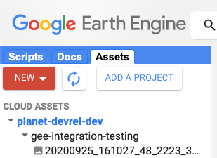
Results in GEE
Now that you’ve delivered your data to GEE, here’s where you’ll find it. Head on over to your GEE console, https://code.earthengine.google.com/, click the “Assets” tab on the left hand side of the screen, and below you will find the Cloud Project you created under the tab called “CLOUD ASSETS”. Under the your Cloud Project name you will find your ImageCollection, and within you will find the images you requested.
Next steps
In this example, we relied on Planet's Google Service Account for data delivery. However, this Service Account is used by many users and may be subject to delays if it reaches its maximum delivery quota. To avoid this, you can create your own Service Account, which would provide you with a dedicated delivery queue and sooner access to your data. In a future blog post, we will discuss the benefits of using a custom Service Account and provide instructions on how to integrate it with your GEE project. Chat with us about any ideas or issues at https://community.planet.com/developers-55. Follow us on Twitter @planetdevs.
The Next Release of the Planet SDK for Python is in Beta
By: Jennifer Reiber Kyle on February 16 2023
The second version of the Planet SDK for Python is in Beta! Install it as a package. Add it to your Conda environment. Install it from the source. And let us know what you think.
Introduction
We are excited to announce the Beta release of version two of our Planet SDK for Python! The Planet SDK (Software Development Kit) for Python is a Python package developed and maintained by the Developer Relations team at Planet. It is version two of what was previously known as the Planet Python Client and works with Python 3.7+. Version two is currently in development and has long been in the works. The beta version has been released and we’re pleased to introduce you to it. This blog post provides an introduction to the Planet SDK for Python and is the first in a blog series which will cover specific aspects of the SDK in more detail.
The Planet SDK for Python is a Python package developed and maintained by the Developer Relations team at Planet. It is version two of what was previously known as the Planet Python Client and it works with Python 3.7+. Currently, it is in development and the beta version has just been released. This blog post provides an introduction to the Planet SDK for Python and is the first in a blog series which will cover specific aspects of the SDK in more detail.
The Planet SDK for Python interfaces with the Planet APIs and has two parts: a Python client library and a command-line interface (CLI). It is free and open source (maintained on github) and available for use by anyone with a Planet API key. It allows developers to automate their tasks and workflows and enables integration with existing processes using Python and more accessible API interactions via the CLI.
In addition to providing Python and CLI interfaces for API endpoints, the SDK also simplifies tasks such as managing paged results, polling for when a resource is ready, and downloading resources. Additionally, it is optimized for fast and reliable http communication. The Python library speeds up complex and bulk operations through asynchronous communication with the servers. The CLI, on the other hand, is designed to fit into complex workflows with piping. These three functionalities will be covered in depth in future posts in this series.
Improvements over version one include a first-class, full-functionality Python library and optimized, robust communication with the servers.
CLI Usage
The CLI is designed to be simple enough to allow for quick interactions with the Planet APIs while also being suitable for inclusion in complex workflows. It supports JSON/GeoJSON as inputs and outputs, which can be provided and handled as files or standard input/output. Here, we demonstrate using the CLI to create and download an order with the Orders API.
Creating an order from an order request that has been saved in a file is pretty simple:
planet orders create order_request.json
The output of this command is the description of the created order. The order id from the description can be used to wait and download the order.
Waiting for the order to be ready and downloading the order is achieved with:
planet orders wait 65df4eb0-e416-4243-a4d2-38afcf382c30 \
&& planet orders download 65df4eb0-e416-4243-a4d2-38afcf382c30
Additionally, the CLI provides support for creating order requests. These requests can be saved as a file or piped directly into the command for creating the order:
planet orders request --item-type PSScene \
  --bundle analytic_sr_udm2 \
  --name 'Two Item Order' \
  20220605_124027_64_242b,20220605_124025_34_242b \
  | planet orders create -
See the CLI documentation for more examples and a code example for how to search the Data API for a PSScene item id for use in defining the order.
Python Library Usage
Planet’s Python library provides optimized and robust communication with the Planet servers. To provide lightning-fast communication in bulk operations, this library is asynchronous. Asynchronous support was added to the Python standard library in version 3.7. Our Python library documentation provides coding examples specifically geared toward the use of the SDK asynchronously. The Python asyncio module documentation is also a great resource.
Here, we demonstrate using the Python library to create and download an order with a defined order request:
import asyncio

from planet import reporting, Session, OrdersClient

request = {
  "name": "Two Item Order",
  "products": [
    {
      "item_ids": [
        "20220605_124027_64_242b",
        "20220605_124025_34_242b"
      ],
      "item_type": "PSScene",
      "product_bundle": "analytic_sr_udm2"
    }
  ],
  "metadata": {
    "stac": {}
  }
}
# use "async def" to create an async coroutine
async def create_poll_and_download():
    async with Session() as sess:
        cl = OrdersClient(sess)

        with reporting.StateBar(state='creating') as bar:
            # create order via Orders client
            # use "await" to run a coroutine
            order = await cl.create_order(request)
            bar.update(state='created', order_id=order['id'])

            # poll...poll...poll...
            await cl.wait(order['id'], callback=bar.update_state)

        # The order completed. Yay! Now download the files
        await cl.download_order(order['id'])

# run the entire coroutine in the event loop
asyncio.run(create_poll_and_download())
The Python library also provides support for creating an order request with the order_request module:
from planet import order_request

item_ids = ["20220605_124027_64_242b", "20220605_124025_34_242b"]

products = [
    order_request.product(item_ids, "analytic_sr_udm2", "PSScene")
]

tools = [
    order_request.reproject_tool(projection="EPSG:4326", kernel="cubic")
]

request = order_request.build_request(
    "Two Item Order, reprojected", products=products, tools=tools)
See the Python library documentation for more examples and a code example for how to search the Data API for the PSScene item ids used in defining the order.
Next Steps
Check it out for yourself! Get instructions on how to install the Planet SDK for Python, learn more about the package, and get plenty of code examples at https://planet-sdk-for-python-v2.readthedocs.io. Browse the source code and track progress at https://github.com/planetlabs/planet-client-python. Check out our Resources Page of Jupyter Notebooks for help getting started. Our Jupyter Notebooks include: Get started guides for Planet API Python Client, Order API & Planet SDK, the Analysis Ready Data Tutorial Part 1: Introduction and Best Practices, and the Analysis Ready Data Tutorial Part 2. Chat with us about any ideas or issues at https://community.planet.com/developers-55. Follow us on twitter @planetdevs.