Forest Carbon Monitoring Technical Specification

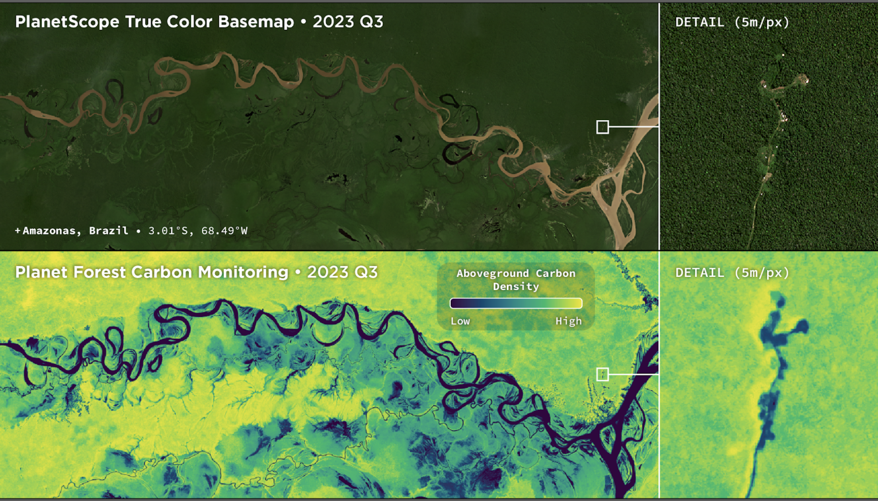
Figure 1: Side-by-side view of PlanetScope Basemaps and aboveground carbon density data over the Amazon River in Amazonas, Brazil.

Overview¶

Forest Carbon Monitoring provides a series of data products for mapping forest change at high resolution worldwide. These products provide timely, operational insights into changes in canopy cover, canopy height, and aboveground carbon density with unprecedented detail, powered by Planet’s unique imaging constellation. The initial release includes quarterly observations starting in December 2020, providing rolling insights into forest structure and carbon.

The Forest Carbon Monitoring products were primarily designed to support project and jurisdictional MRV¹, as well as supply chain risk evaluations for EUDR² compliance. The leading project type in carbon markets follows the REDD+³ framework of avoiding deforestation, and Forest Carbon Monitoring excels at tracking forest loss at fine scales and quantifying the resulting carbon losses.

The power of quarterly, high resolution data is in detecting complex, diffuse patterns like degradation and regrowth. Not all forest loss is uniform, and it is crucial to map the selective harvests of individual trees or small groups of trees in order to accurately estimate forest inventories at scale.

While detecting changes early in a tree's life history is often challenging, Forest Carbon Monitoring is sensitive to young tree growth. These data can be combined with in situ data for digital MRV of natural regeneration or explicit ARR⁴ interventions.

When scaled up to sub-national or national scales, Forest Carbon Monitoring can support jurisdictional carbon accounting and policy implementations related to land-based climate mitigation.

Product Specifications¶

Table 1: Forest Carbon Monitoring product specification

Specification	Value
Metrics	Canopy cover, canopy height, aboveground carbon density
Spatial extent	Global land mass > -60S and < 75N, excluding ice sheets
Temporal extent	Dec. 2020 - Present
Temporal resolution	Quarterly
Temporal periods	Q1: Dec 21 - Mar 20
	Q2: Mar 21 - Jun 20
	Q3: Jun 21 - Sep 20
	Q4: Sep 21 - Dec 20

Canopy cover (CC) quantifies the percentage of area occupied by trees within a pixel, where a tree is defined as vegetation 5 meters or taller. This metric will be most sensitive to tree loss events like timber harvest or deforestation, and to increases in tree cover due to regeneration or ARR.

Canopy height (CH) quantifies the average top-of-canopy height within each pixel. While this metric is sensitive to tree loss, it is less sensitive to large tree growth. Vertical growth is typically slower in mature trees compared to young trees, meaning quarter-over-quarter height increases are not frequently observed outside of regrowth contexts.

Aboveground carbon density (ACD) quantifies the expected density of carbon stored in woody biomass, measured in units of mass per area (megagrams of carbon per hectare). It is not a direct estimate of the total carbon in each pixel or each tree, but an estimate of area-based carbon density.

Asset Properties¶

This tables specifies the properties of the data assets delivered by the Planet Subscriptions API.

Table 2: Forest Carbon Monitoring data resource properties

Metric	Asset Name	Units	Type	Typical Range	No Data Value	Band Count	Resolution
Canopy Cover	cc	%	UINT8	0 - 100	255	1	0.000025° (±3x3 m)
Canopy Height	ch	m	UINT8	0 - 50	255	1	0.000025° (±3x3 m)
ACD: Minimum Mapping Unit	acd-mmu	Mg/ha	INT16	0 - 300	32767	1	0.00025° (±30x30 m)
ACD: Downscaled	acd	Mg/ha	INT16	0 - 300	32767	1	0.000025° (±3x3 m)
CC Uncertainty	cc-uc	%	UINT8	0 - 100	255	2	0.000025° (±3x3 m)
CH Uncertainty	ch-uc	m	UINT8	0 - 80	255	2	0.000025° (±3x3 m)
ACD MMU Uncertainty	acd-mmu-uc	Mg/ha	INT16	0 - 300	32767	2	0.00025° (±30x30 m)
ACD Downscaled Uncertainty	acd-uc	Mg/ha	INT16	0 - 300	32767	2	0.000025° (±3x3 m)

Aboveground carbon density data are provided at two spatial resolutions.

The 30m Minimum Mapping Unit (MMU) data estimates carbon density at the native resolution of the model. This product is straightforward to analyze and validate, and aligns with best mapping practices recommended by the Committee on Earth Observing Systems (CEOS).

The 3m Downscaled product provides carbon estimates that match the resolution of the canopy height and canopy cover products. The value of downscaled data is to quantify carbon density over small—but not sub-tree—areas, like smallholder farms, selective harvests, field plots, and carbon projects.

Because the downscaled data are provided at a spatial resolution finer than the size of most tree crowns, downscaled carbon estimates should be aggregated across multiple pixels, which greatly improves prediction quality and interpretability. This product empowers users to flexibly aggregate data to the scales that fit their needs, particularly in use cases where coarse, gridded data pose analytical challenges. See the Carbon Downscaling Method section for more details on the downscaling approach, and the Minimum Mapping Units section for guidance on aggregation.

Table 3. Uncertainty band descriptions

Uncertainty band	Description
Q05 (band 1)	Lower prediction bound (5th percentile)
Q95 (band 2)	Upper prediction bound (95th percentile)

Uncertainty data are provided as calibrated 90% prediction intervals for each pixel in each quarter. These values are provided in the same units as their respective reference data. In other words, the pixel values and units are consistent between the "cc" and "cc-uc" assets.

Input Data¶

Canopy height and canopy cover are estimated at high resolution using computer vision models. Airborne LiDAR data are the response variables, and a series of satellite-derived datasets are the feature variables.

Forest carbon density is first estimated at 30m resolution using a gradient boosting regression model, then downscaled using a linear downscaling model. GEDI L4A data are the response variable, and canopy height, canopy cover, and elevation data are the feature variables.

Table 4: List of inputs for Forest Carbon Monitoring production

Product	Description
Airborne LiDAR	Point cloud data processed to rasters of canopy height and canopy cover at 1m resolution, then resampled to match the Surface Reflectance data.
GEDI L4A	GEDI L4A data encode modeled estimates of aboveground biomass density across most of the terrestrial biosphere.
Surface Reflectance	Quarterly, 4-band PlanetScope Surface Reflectance Basemaps, spectrally normalized to Sentinel-2.
Forest Carbon Diligence	30m canopy height and canopy cover data from the Forest Carbon Diligence product.
Digital Elevation Model (DEM)	Copernicus GLO-30 DEM are used for most of the global landmass, ALOS AW3D30 is used where GLO-30 does not provide data.

Methods¶

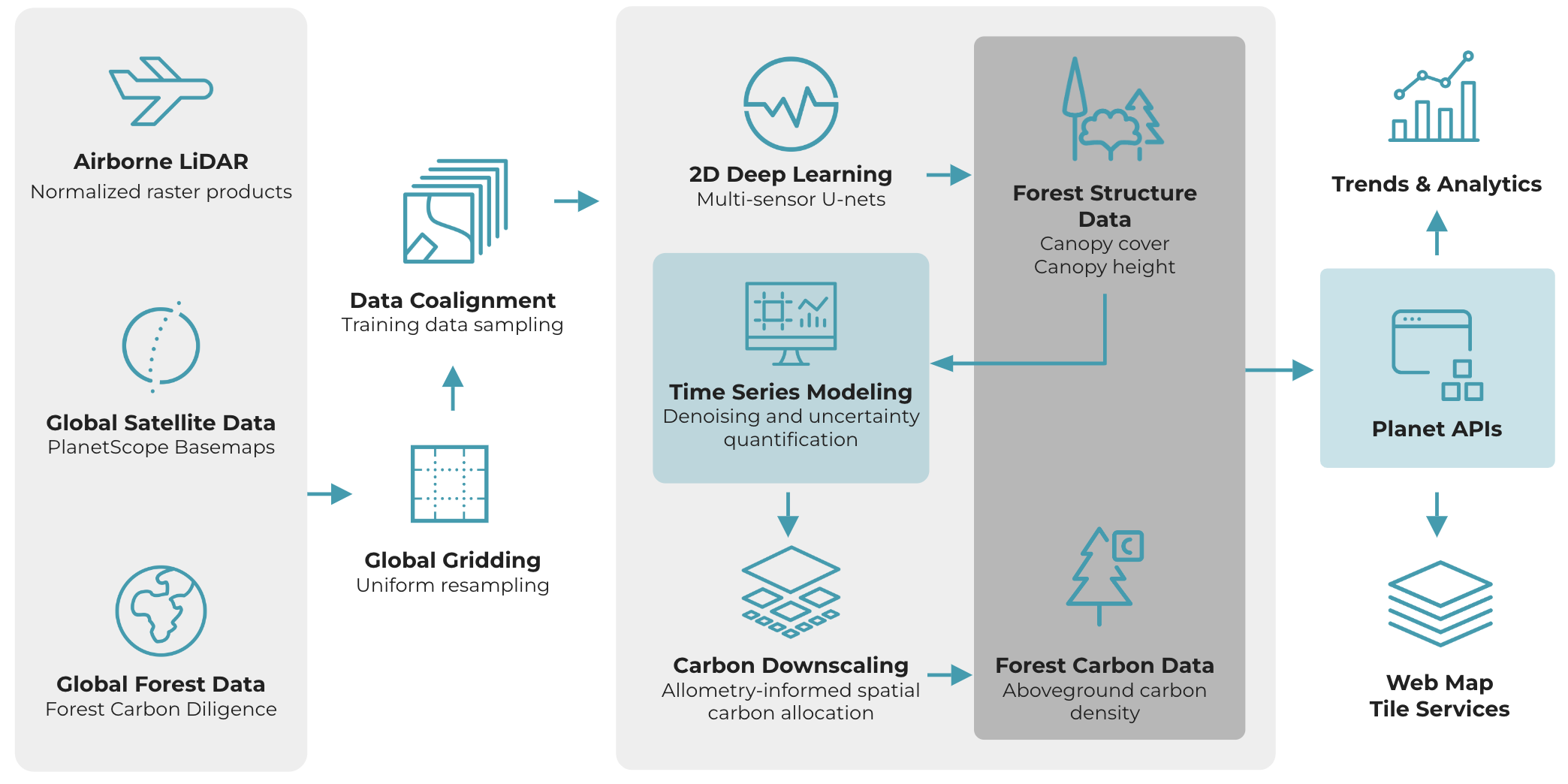Figure 2: Workflow diagram for Forest Carbon Monitoring illustrating the flow of data for delivery.

Global Gridding and Co-alignment¶

A global grid was used to create deterministic, geographically independent samples, assigned to non-overlapping sets for model training, validation, and testing.

This grid was specified using the EASE Grid 2.0 equal area projection (EPSG:6933) at 3.4m resolution. EASE Grid offers an efficient layout design, storing only 60% of the pixel count compared to a geographic coordinate system at a comparable resolution. This cylindrical projection preserves area but distorts shapes close to the poles, which could introduce spatial artifacts in the vision model. A large amount of training data was acquired at high latitudes to mitigate this effect.

Training data was generated by randomly sampling 128x128 pixel tiles from regions with high quality airborne LiDAR data, and a deterministic grid was used to define the sampling strategy. First, the grid was overlaid with the LiDAR extent, and tile centroids were sampled over non-overlapping valid data locations.

Once the tile locations were selected, a coarser grid was used to split data into training, validation, and testing groups. 2x2 quads were split so that samples within two of the tiles were used for model training, one for validation, and one for testing. This resulted in an approximately 50-25-25 split with no spatial overlap between tiles. In total, this produced 27.5 million hectares of data for training and evaluation, with 806,826 samples used for training, 253,497 for validation, and 352,870 for testing.

Quarterly, 4-band surface reflectance mosaics were produced starting in 2018 based on the quality and quantity of available PlanetScope data. Surface reflectance and LiDAR data were time matched to select temporally-coincident observations. LiDAR data collected prior to 2018 was matched to the 2018 surface reflectance mosaic. For LiDAR data with large or imprecise collection periods, the nearest leaf-on quarter was selected (corresponding to spring in the northern and southern hemisphere).

Training data were spatially resampled to align in shape and resolution. Each sample was a 128x128 array at 3.4m resolution, projected to EASE Grid. The response data—LiDAR-derived canopy height and canopy cover—were average resampled to this scale. The feature data—surface reflectace mosaics and the 30m Forest Carbon Diligence data—were extracted with nearest-neighbor resampling then concatenated in the channel dimension, creating a 6-band feature stack. Diligence data from the time-matched year was selected for each sample. The Diligence data were included to provide contextual information to the model regarding the absolute canopy height and canopy cover values for each sample, and to improve alignment across products.

2D Deep Learning¶

U-Net image regression models were trained to predict canopy height (m) and canopy cover (%) at 3.4m resolution, using surface reflectance mosaics and 30m maps of height and cover as predictors.

The height and cover response datasets were modeled simultaneously in a multi-task learning framework using Joint Task Training (Crenshaw 2020). This approach optimized both accuracy and efficiency. There is strong but non-linear covariance between canopy height and canopy cover, and many of the spectral features used to estimate these patterns are shared across contexts, leading to efficient model training convergence.

Including canopy height and canopy cover maps from the Diligence product increased the overall feature dimensionality, improving predictive power. Sharing a joint encoder/decoder also improved consistency in the output prediction features, so post-processing harmonization was unnecessary. Multi-task learning reduced the overall saturation of canopy height predictions, increasing the predicted heights at the tall end of the distribution, though these effects are still pronounced.

The U-Net model architecture was modified to include ResNet blocks and a series of network-in-network connections (Lin et al. 2013, Zhang et al. 2018). The Log Cosh loss function was used to minimize the contributions of large residual errors to model convergence, which was found to improve canopy height predictions. Using spatially-independent validation data—instead of shuffling training and validation data at runtime—was found to improve model generalization, minimizing the difference between training and testing metrics.

Model inference was applied independently to each quarter's feature stack. As a result, seasonal vegetation patterns and sun-sensor observation variability introduce quarter-over-quarter variance to the raw model predictions. Experiments found that training models with just leaf-on observations improved generalization across quarters, compared to models trained using both leaf-on and leaf-off observations. This quarter-over-quarter variance is addressed downstream using time series models.

Time Series Modeling¶

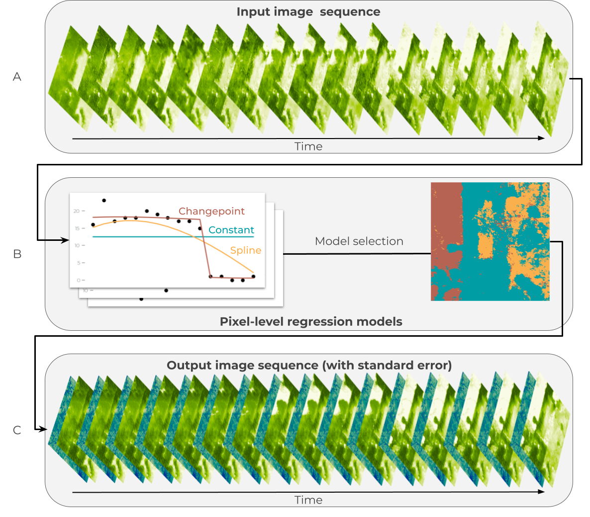Figure 3: Statistical modeling for estimating canopy height and canopy cover over time. (A) An image time series is generated from the raw predictions of the vision model for times t=1, … T. (B) Three regression models are fit for each pixel: a constant model to represent the temporal mean (blue), a changepoint model to represent sudden change (red), and a spline model to represent gradual change (orange). A model is selected for each pixel, with the preferred model color coded in the image on the right. (C) The preferred model for each pixel is used to generate denoised predictions for each time step: expected values (green color ramp) and standard errors of the predictions (blue color ramp).

The vision model predicts height and cover for each quarter independently, and the predictions contain variation related to phenology, illumination, and sensor calibration. We minimize the variation in prediction sequences using statistical models.

For each pixel, three models are fit:

1. A constant-in-time model, which represents stability over time
2. A spline model, which represents gradual change
3. A changepoint model, which represents fast change

The constant-in-time model assumes that all variation in predictions is due to noise. This model is expected to perform well when height or cover remains stable over time or when changes are minimal relative to the noise in the predictions (e.g., slow growth that is not detectable over a few years).

The spline and changepoint models are designed to capture slow and fast changes, respectively. Regularized B-splines are used to estimate non-linear trends, while the changepoint model includes a discrete change point parameter at the timestep with the greatest change in predicted height or cover.

The preferred model for each pixel is selected using Akaike's Information Criteria (AIC). An additional heuristic is applied to reduce noise: if the coefficient of variation (over time) for the preferred model's predictions is below a threshold, the constant-in-time model is selected. This coefficient of variation threshold is a hyperparameter tuned alongside the AIC threshold.

Once a preferred model is selected for each pixel, predictions are generated and predictive error is quantified using the standard errors of predicted values from the regression models. These standard errors are used downstream to quantify pixel-level uncertainty for height and cover.

Carbon Downscaling¶

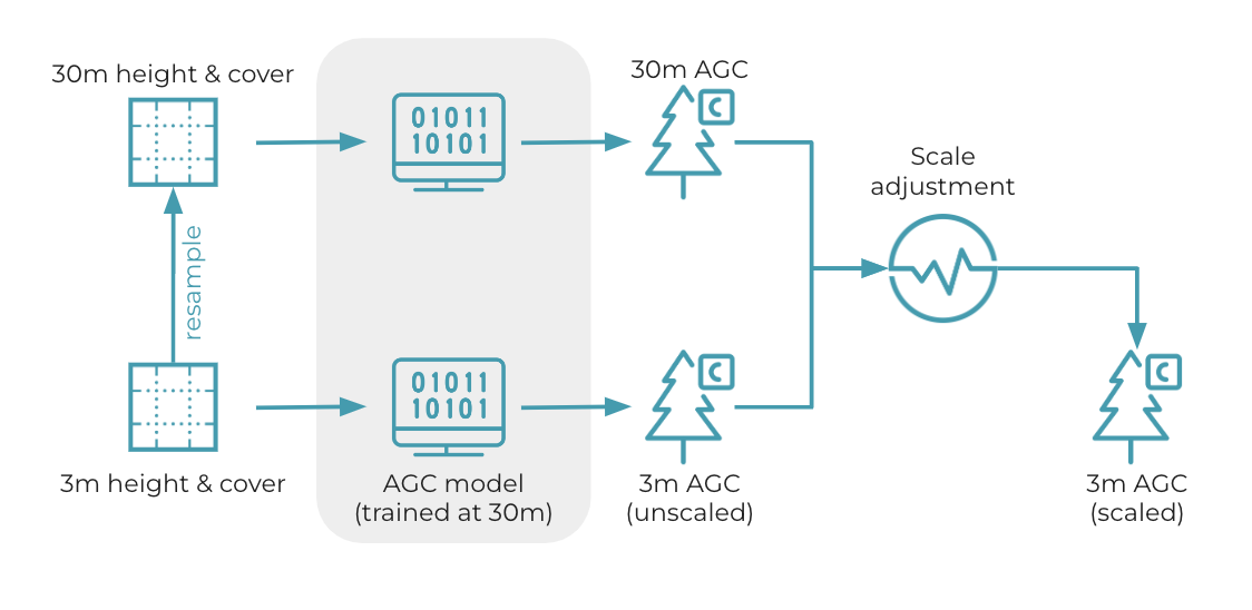Figure 4: Overview of 3m aboveground carbon estimation. First, 3m height and cover data are average resampled to 30m. The 3m and 30m data are then provided separately as inputs to the AGC model (natively trained at 30m). This produces 3m and 30m carbon predictions. To ensure that the average of 3m AGC data equals the average of the 30m data, we apply a scale adjustment to the 3m data based on the ratio of 30m and unscaled 3m means.

Aboveground carbon density estimates are generated at 3m nominal resolution using statistical downscaling. This downscaling approach is designed to satisfy two criteria:

1. At fine scales, carbon estimates should be consistent with 3m height and cover.
2. At large scales, aggregated 3m carbon estimates should be consistent in expectation with 30m carbon estimates.

Simple linear downscaling of a model trained at 30m is used to meet these criteria. This 30m model is trained on L4A aboveground biomass estimates derived from NASA's Global Ecosystem Dynamics Investigation (GEDI) spaceborne lidar sensor. Given height and cover estimates, the model can predict aboveground biomass, which is converted to aboveground carbon by multiplying by a scalar representing the global mean carbon concentration. The details on model training, model performance, and scaling is described in more detail in the Forest Carbon Diligence Technical Specification. 30m is considered the "native scale" of the carbon model.

To create 3m estimates from the 30m model, 3m height and cover are passed as inputs, generating raw 3m carbon predictions. These predictions are "raw" due to the scale mismatch between the model's training resolution (30m) and the deployment resolution (3m). Next, 3m height and cover are average resampled to 30m, and the 30m height and cover inputs are passed to the model to create 30m carbon estimates at the native resolution. Mean carbon is then computed for both the raw 3m and native 30m predictions, and the ratio of means is used to compute a scale adjustment. Final 3m carbon predictions are computed by scaling raw 3m carbon estimates, ensuring that the average carbon of the 30m predictions equals the average carbon of the final 3m predictions.

Pixel-level Uncertainty¶

Standard errors from the pixel-level time series models are used to construct 90% prediction intervals for height and cover.

Intervals are constructed as:

where \(y_{\text{pred}}\) is a predicted value from the time series model, \(\sigma_{\text{pred}}\) is the standard error of the prediction, and \(\widehat{q}\) is a parameter estimated using withheld data via split conformal inference.

Split conformal inference uses disjoint partitions of a dataset to produce well-calibrated prediction intervals. These are 90% prediction intervals that contain the true value approximately 90% of the time (Angelopolous and Bates 2021).

A calibration dataset is used to estimate \(\widehat{q}\), a scalar quantity that determines the width of the interval relative to the standard error to achieve 90% coverage. After generating predictions with \(\widehat{q}\), empirical interval coverage is quantified on a spatially non-overlapping test set. Test set coverage was 90.3% for canopy cover and 91.7% for canopy height.

Data Quality¶

Deep Learning Model Performance¶

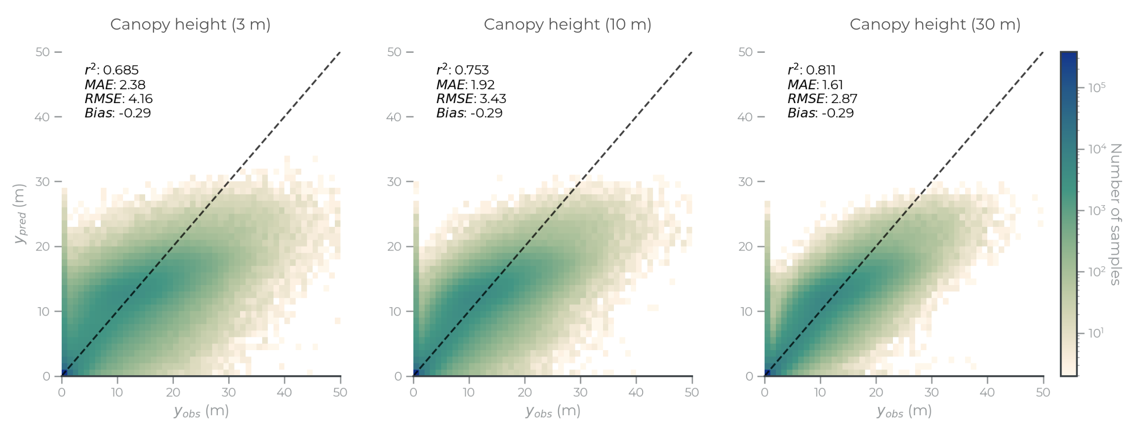Figure 5: Scatter plots for canopy height predictions at 3m (left), 10m (middle) and 30m (right) resolutions.

There are several drivers of prediction uncertainty, including model variance, observation quality, and orthorectification quality. These drivers are difficult to disentangle, but we provide a comparison of multi-scale model performance below to illustrate how model performance improves with aggregation.

Users are encouraged to analyze the data at the scale that fits their analysis. This is often at the original scale of the data. But in contexts where prediction accuracy is critical, aggregating forest structure data provides meaningful improvmeents. High resolution data is valuable beyond providing detailed maps; aggregating high resoultion data can capture subtle, fine-scale dynamics more precisely at scale than direct observations at lower resolution.

Table 5. Multi-scale model performance comparison

Metric	Resolution	R2	MAE	RMSE
Canopy height	3m	0.68	2.4m	4.2m
	10m	0.75	1.9m	3.4m
	30m	0.81	1.6m	2.9m
Canopy cover	3m	0.70	12%	20%
	10m	0.78	9%	16%
	30m	0.84	7%	12%

Canopy Height Saturation¶

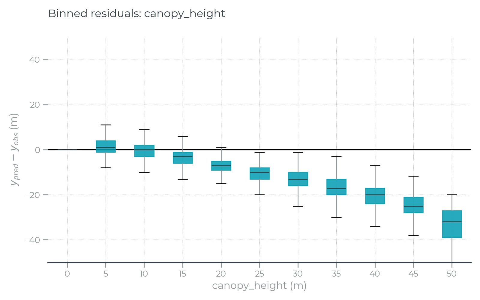Figure 6: Binned residual error plots for canopy height show attenuated signal for taller trees. The residual errors for each test data observation were binned in 5 meter increments for this box plot, showing canopy height predictions are systematically lower for tall trees. This plot is not normalized by sample frequency.

Signal saturation is a well-known challenge to estimating canopy height using optical satellite data (Mutanga et al., 2023). This refers to the limited signal available in optical remote sensing data to predict tree heights beyond 25-30 meters above ground. While several modeling approaches were tested to minimize this effect (see 2D Deep Learning), it remains visible in the residual error plots (Figure 6). This might pose a challenge for users who depend on unbiased canopy height estimates (in allometric regression models, for example).

In empirical use cases, signal saturation may not be as problematic. For example, the aboveground carbon density model used in this product estimates empirical relationships between predicted canopy height and canopy cover maps and the observed carbon density data. Practically, this results in strong model performance for the low and mid range of carbon estimates, though predictions in the most carbon-dense forests will likely be underestimated.

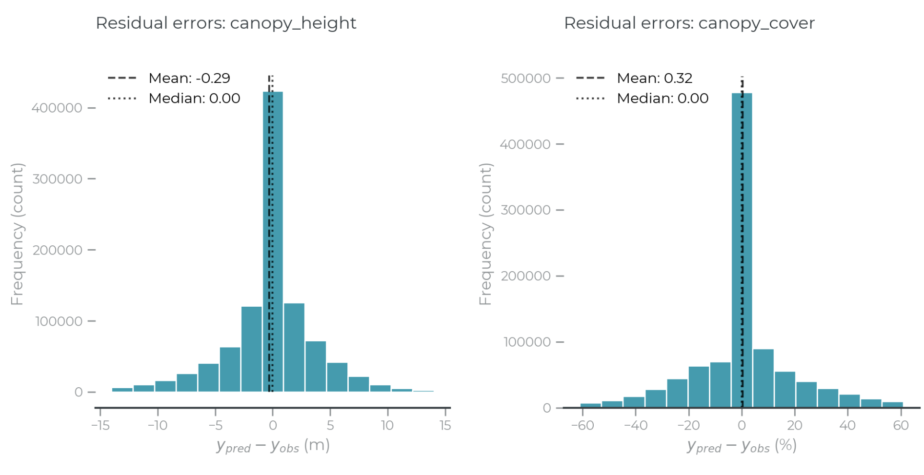Figure 7: Residual error histograms for canopy height (left) and canopy cover (right).

Overall, the deep learning model converged to predict both canopy height and canopy with low total bias across the full test data set. Although there is signal saturation among taller trees, higher predictions at lower heights balance the overall predictions, driving low population-level bias.

This effect further demonstrates the value of spatial aggregation. While bias may occur at any one point across the landscape, these biases decrease with aggregation, and the total bias over large areas is likely to be low.

Minimum Mapping Units¶

The aboveground carbon density products are provided at multiple spatial resolutions: 30m and 3m. The reason for providing multiple assets is related to a geographic concept known as the minimum mapping unit. Knight and Lunetta, 2003 provide a short review of this topic.

The minimum mapping unit for forest carbon products refers to the smallest area over which carbon estimates can be reliably quantified and validated. Because the forest carbon data were fit using GEDI L4A data and 30m feature data, the minimum mapping unit for the carbon model is 30m. This is approximately the size of a 0.1 ha field plot. Although the downscaled product is provided at 3m resolution—which can be smaller than the size of an individual tree—the minimum mapping unit for analysis remains 30m.

So why provide a data product at a scale finer than the minimum mapping unit?

The primary value proposition of high resolution data is to provide a flexible data product that can be aggregated to the appropriate scale of analysis, which varies by use case.

Current best practices recommend mapping carbon at 0.25 - 1 ha (50 - 100m) resolution in tropical forests, and 0.1-0.25 ha (30 - 50m) in boreal and temperate forests (CEOS 2021, Frazer et al. 2011). The Food and Agriculture Organization (FAO) developed a consensus forest definition, which specified minimum thresholds of areas with 10% canopy cover, 5 m tree height, covering at least 0.5 ha (FAO 2000). Aggregation to 1 ha has been shown to minimize prediction uncertainty and identified as the optimal scale for accurately estimating forest carbon stocks from remote sensing (Mascaro et al. 2011, Chen et al. 2016).

While each of these scales is greater than the 0.1 ha minimum mapping unit, data provided at that resolution may still prove prohibitive. Scale mismatches between field and satellite datasets has long been one of the primary drivers of uncertainty and barriers to effective validation, especially when validating plots that may only be one or two pixels in size or fall on borders between pixels (Wu and Li, 2009, Anderson 2018, Réjou-Méchain et al. 2019). Mismatches between satellite resolution and forest definitions make global forest change analysis prohibitively complex, too. This has become so acute that some researchers have called to change the FAO's global definition of forests to instead be defined by the 30m resolution of Landsat (Zalles et al. 2024).

Instead of asking users to redefine their problems to accomodate their data, the downscaled product was developed to accomodate the wide range of contexts our users work in. It is straightfoward to resample the downscaled product over field plots, carbon projects, disturbed areas, or tree planting sites. The carbon estimates will be valid so long as the data are aggregated to at least the minimum mapping unit.

To demonstrate the value of high resolution carbon data, consider the case of carbon quantification over smallholder farms. Recent work found that smallholder farmers in Rwanda planted an average of 3 trees per farm over a decade of analysis, which added up to over 50 million new trees nation-wide (Mugabowindekwe et al. 2024, Brandt et al. 2024). Individually, these contributions to a national carbon budget are minimal, and may not be detectible from lower resolution observations. But a full accounting of smallholder contributions could prove meaningful at jurisdictional scales. Developing cost-effective MRV tools for quantifying changes in carbon stocks was identified as a top priority for engaging smallholder farmers in carbon markets, and high resolution data uniquely addresses this need (Schilling et al. 2023).

The 3m downscaled forest carbon product was not developed to provide sub-tree estimates of carbon density; it was designed to empower users to flexibly aggregate data to the scales that fit their needs, particularly in use cases where coarse, gridded data pose analytical challenges. The 30m MMU product supports direct carbon stock analyses, requiring no additional modifications by uses to derive meaningful carbon estimates. Both products should be analyzed at a minimum mapping unit of 30m, though that does not preclude aggregation to the appropriate scale of analysis for your use case.

Known Issues¶

Halo effects. The time series model estimates forest structure patterns across the full temporal extent of data and updates all predictions simultaneously. This can create visually-distinct boundaries between areas where rapid changes were observed, which propagate back in time. As a result, post-change edge effects can appear in the data prior to the observed vegetation change. This will typically be captured by the pixel-level prediction intervals, showing higher prediction uncertainty on the borders of disturbances. Anecdotally, this effect appears to be largely visual, with low numerical differences.

Pixel coregistration. PlanetScope surface reflectance data are provided with some positional uncertainty, meaning pixel locations may shift slightly quarter-over-quarter. PlanetScope absolute positional uncertainty is quantified in Section 3.3 in the Imagery Product Specification. Practically, this presents as a slight decrease in pixel-level contrast, and predictions may not appear as crisp as expected.

False positive changes in the most recent time step. The time series model is an effective outlier filter, smoothing over noisy observations from unmasked clouds, snow, or missing data. These models rely on additional observations that follow the noisy observations, which indicate a change did not persist. Additional observations are not available for the most recent time step, which increases the rate of false positive changes. For time-sensitive use cases, we advise users to consult the uncertainty layer, which should show high uncertainty in areas with anomalous change. For less time-sensitive use cases, we advise using the previous quarter's data to minimize false positives. The most recent quarter's data will be updated once new observations are available to correct these issues.

Most changes are observed at year-to-year boundaries. Including the annual, 30m Forest Carbon Diligence data as predictive features improves prediction accuracy but introduces a temporal mismatch in production. New Diligence observations are included at Q1 of each year, but are not updated for each following quarter. Changes detected from Diligence—both growth and loss—may not be captured until the next year. This means that change detection primarily occurs at year-to-year boundaries when new 30m observations are included.