Viewing a Flood Event with the Planet Explorer QGIS Plugin

Time to complete: this tutorial is expected to take anywhere from 30 minutes to 2 hours depending on your QGIS and satellite imagery familiarity.

IT’S INSTALL TIME¶

First things first, you will need to purchase a Planet subscription here or sign up for Planet's Developer Program. The Planet QGIS Plugin can be installed, but not used, until you log in with your Planet account. Additionally, some functionality such as imagery download may be limited with a Developer Program account.

Second, if you don’t already have QGIS, download and install it by going to Download QGIS. Most likely you will want to use the QGIS Standalone Installer rather than the OSGeo4W Network Installer. Planet's QGIS plugin is designed to work on QGIS versions 3.6+. Remember that you can have concurrent QGIS installs of different versions on the same machine, so if you haven’t upgraded in a while, it would be best to get the latest version, without fear of ruining older projects or needing to uninstall older versions.

Once installed, start up QGIS Desktop (you can choose the with GRASS version or the one without). In the QGIS menu bar, select the Plugins drop-down, then select All if it isn’t already selected, and type “Planet Explorer” in the Search… box. Select it in the list and press Install Plugin. A new button is added to the toolbar. Your QGIS may look different than the one below depending on the version and which panels and toolbars are open but the general process should be the same.

Note: if an Enter Credentials window pops up, put in your Planet login password twice and press OK.

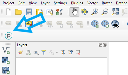
Press the Planet Explorer button that now appears in the QGIS Toolbar section. Note that your button may appear in a different place depending on your past toolbar configurations.

Once you press the button the Planet Explorer Panel will appear, located on the right-hand side of the QGIS window. Note that if you already had one or more panels open on the right-hand side of your QGIS window from previous QGIS sessions, the Planet Explorer Panel will appear at the lower-right, underneath them.

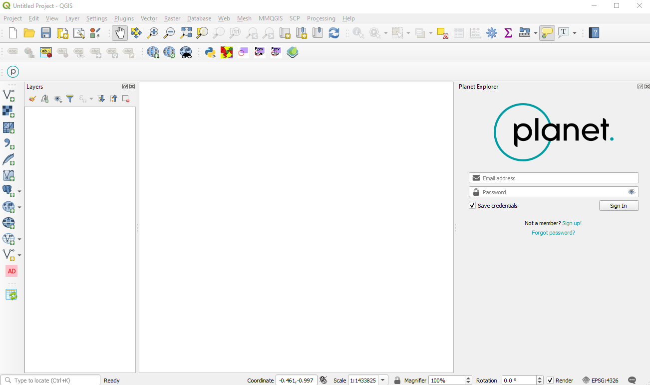
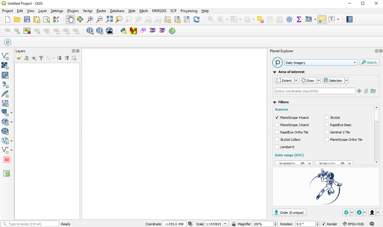
Use the Email address and Password input boxes to input your credentials if you already have them. If you do not have them and would like to sign up for Planet's Developer Program, use the Sign up! link, sign up, and then return here and input your credentials. Once authenticated, the Planet Explorer Panel will look like this:

If you ever close the Planet Explorer Panel and want to get back to it, simply click on View in the menu bar, then Panels, and then check the box next to Planet Explorer.

IT’S CRAZY QUICK TIME¶

Sometimes people want to jump right in. If that sounds like you, use this section as your 30-second quick-start and then proceed to the tutorial. Otherwise, skip to the tutorial.

1. Add a dataset to QGIS
2. Click Extent > Current visible extent in the Planet Explorer Panel
3. Click Search
4. Under Date acquired, check one of the checkboxes. Next to it, press the sunburst Settings button and choose Add preview layer to map.

IT’S TUTORIAL TIME¶

Flooding occurred along the Missisquoi River, Vermont in early November 2019. Let’s take a look at what happened there by exploring a location that was affected: Richford, Vermont. We’ll see what satellite imagery is available before and during the flood, which took place on and around November 1, 2019. We’ve extracted some village points in Northern Vermont from OpenStreetMap and prepared them in a geojson file called village-points.geojson, located in this directory. Download that file and drag and drop it onto the QGIS Layers Panel.

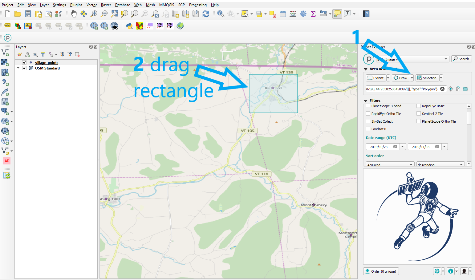
Use the Draw > Rectangle button in the Planet Explorer Panel to draw a rough rectangle around the point representing Richford, which is the northernmost point in this dataset. To do this, make sure to keep the mouse button pressed while clicking and dragging the rectangle onto the QGIS map window. Note: we used the QuickMapServices plugin for QGIS to add a basemap to the project. This is optional.

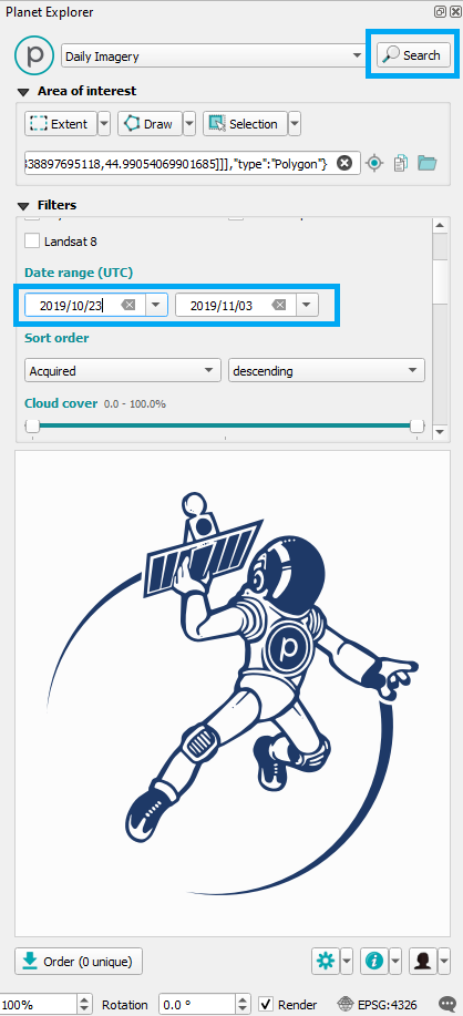
The map automatically zooms to this location and places a blue dashed line around it. This indicates the search area, also called Area of Interest (AOI). Next, because we want imagery from a specific time period, use the Date range (UTC) input boxes to provide two dates: 2019/10/23 and 2019/11/03. These are found in the Filters section of the panel. You may have to scroll the Filters section down to see the Date range (UTC) input section, depending on how much screen space is available for you. Then click Search.

A few PlanetScope 4-band Scenes appear under the Date acquired section. Hover over those scene listings and notice that blue lines appear on the map. These show you where, exactly, the satellite captured imagery on that date. Depending on the initial size of your search rectangle, you may want to zoom out a bit in order to see the entirety of the PlanetScope imagery footprints.

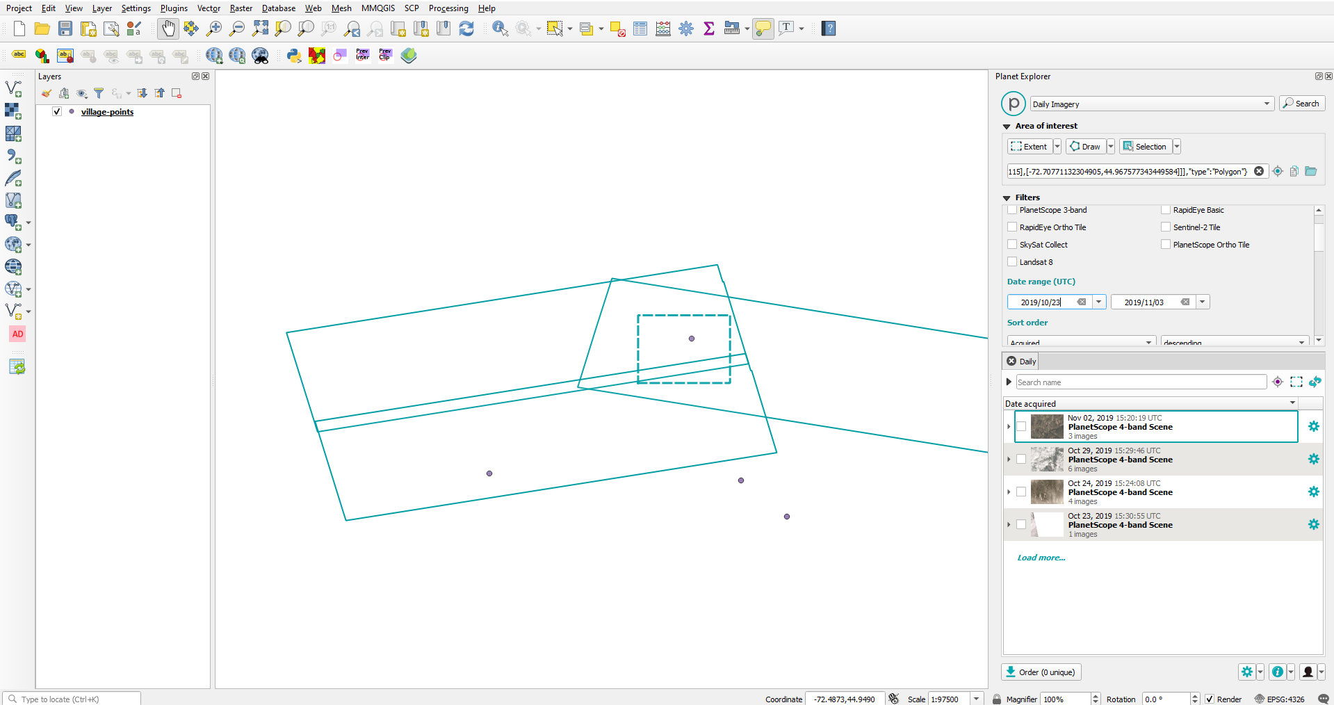
The image thumbnail next to each scene will also give you a sense of the general amount of cloud cover in the scene. While your list of available scenes may look different depending on the size of the rectangle you drew, in our case the first and third scenes in our list look cloudy.

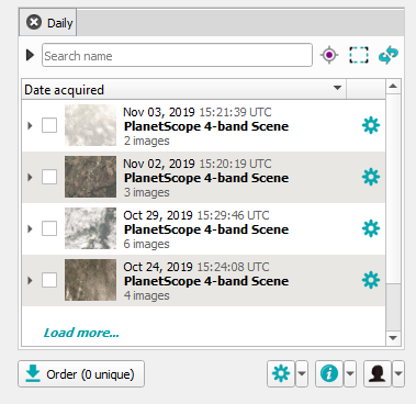
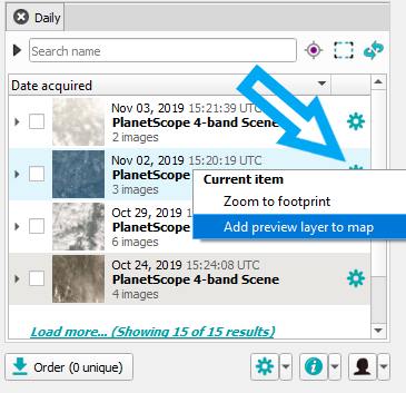
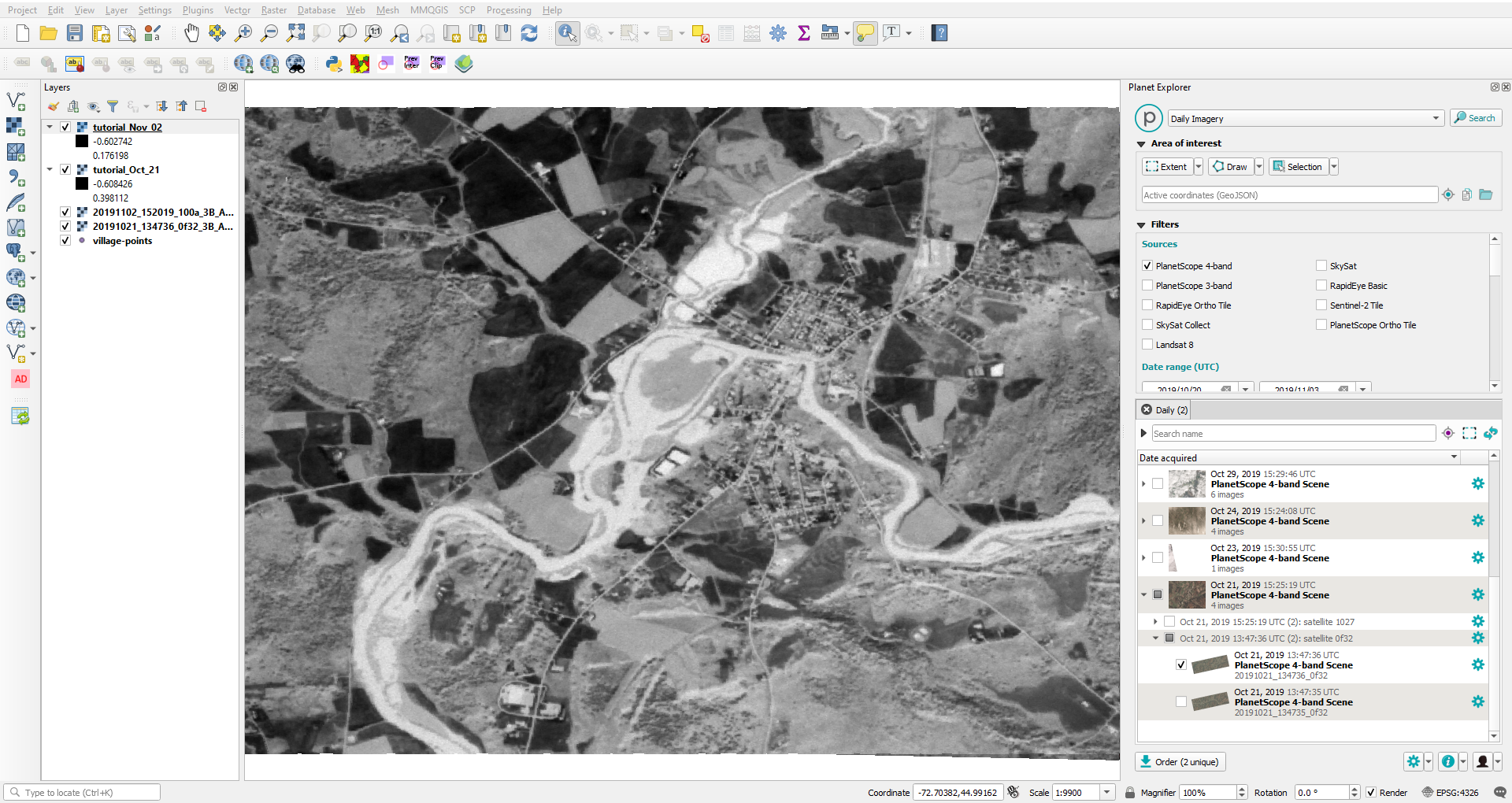
To see the two less cloudy images in the big map view, click the blue sunburst settings button to the right of each of them, and click Add preview layer to map. Please look closely at the following screenshot so that you can try and add the same two scenes to your map, since your list may differ from ours. Specifically, we are adding the Nov 02, 2019 and Oct 24, 2019 scenes.

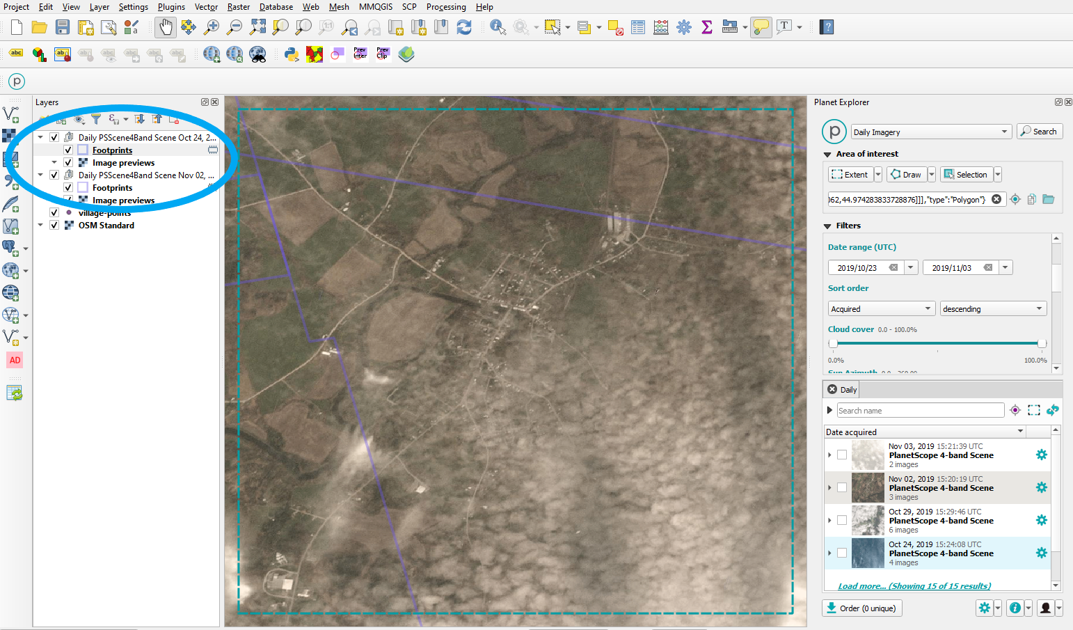
Notice that the QGIS Layers Panel now lists those two scenes as image previews. You can turn them on and off in the Layers Panel and pan and zoom the map to examine them.

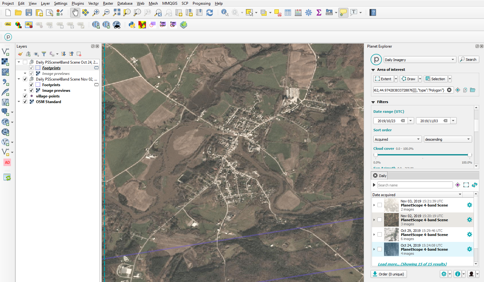
Zoom the map into the town of Richford with the Nov 02, 2019 Image preview clicked on but the Oct 24, 2019 Image preview clicked off. You can see some of the flooding during this "Halloween" storm in the map now:

That Nov 02, 2019 image is fairly clear. However, if you click on the Oct 24 image you may notice that it looks too cloudy. Since this Oct 24 scene was going to be our before image, it is probably okay to expand our date search to a slightly earlier time frame to see if we can get a better before image.

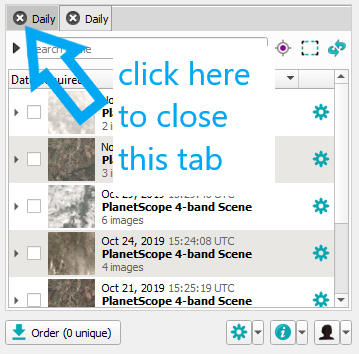
Change the first date in the Filters section to 2019/10/20 and press Search again. A new tab appears in the results area with the new search results. Add the Oct 21, 2019 scene as a preview to the map, just as we did with the other two images. This one is mostly cloud-free and will work as our before image. Close the first results tab so that just the one results tab is open:

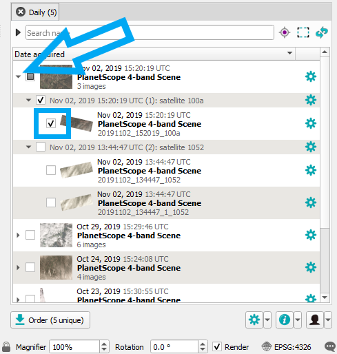
It's now time to place an order to get the imagery since we were just looking at previews up until now. Ordering an image will make it available for download, where we can run more advanced analysis on the GeoTIFF. Expand the November 2 scene listing to see that there are actually three images that we could order. Click the checkbox next to the image with the “100a” suffix.

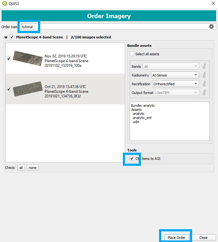
Expand the October 21 scene listing as well and expand the image listing with the “0f32” suffix. Click the checkbox next to the listing 20191021_134736_0f32. Now click the Order button to open the order dialog. Add a name for the order and check Clip items to AOI to clip them automatically to our location. Click Place Order.

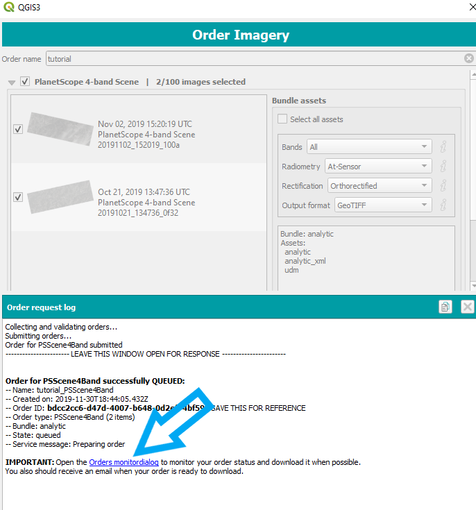
Notice that the bottom of the dialog now shows an order request. Click the link provided to open your Orders monitor dialog.

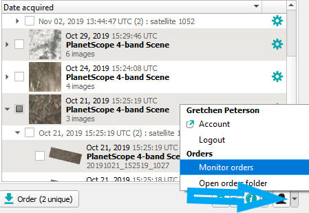
This will show the status of your previous orders as well as this new order. You can always get to the Orders monitor dialog again if you close it, via the User Menu button at the lower-right corner of the Planet Explorer panel shown here:

Once the order status is complete the download button will be activated when you press Refresh.

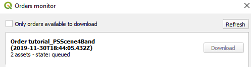
You will also be notified by email that the order is ready and you can download it directly from the provided email link if you prefer.

If the preview scenes from earlier in our explorations are still in your QGIS project, remove them by right-clicking on them and choosing Remove. This will keep the project easier to work with.

Download the zip file in the Orders monitor, unzip it, and add the scenes to QGIS by dragging and dropping the two <.tif> files with the largest sizes to the QGIS Layers Panel. Note, after unzipping the download, the data will be in a sub-folder called files. These files are called:

    20191021_134736_0f32_3B_AnalyticMS_clip.tif
    20191102_152019_100a_3B_AnalyticMS_clip.tif

Notice that the first one is the October 21 dated scene, which is apparent from the beginning of the file name, and the second is the November 2 dated scene.

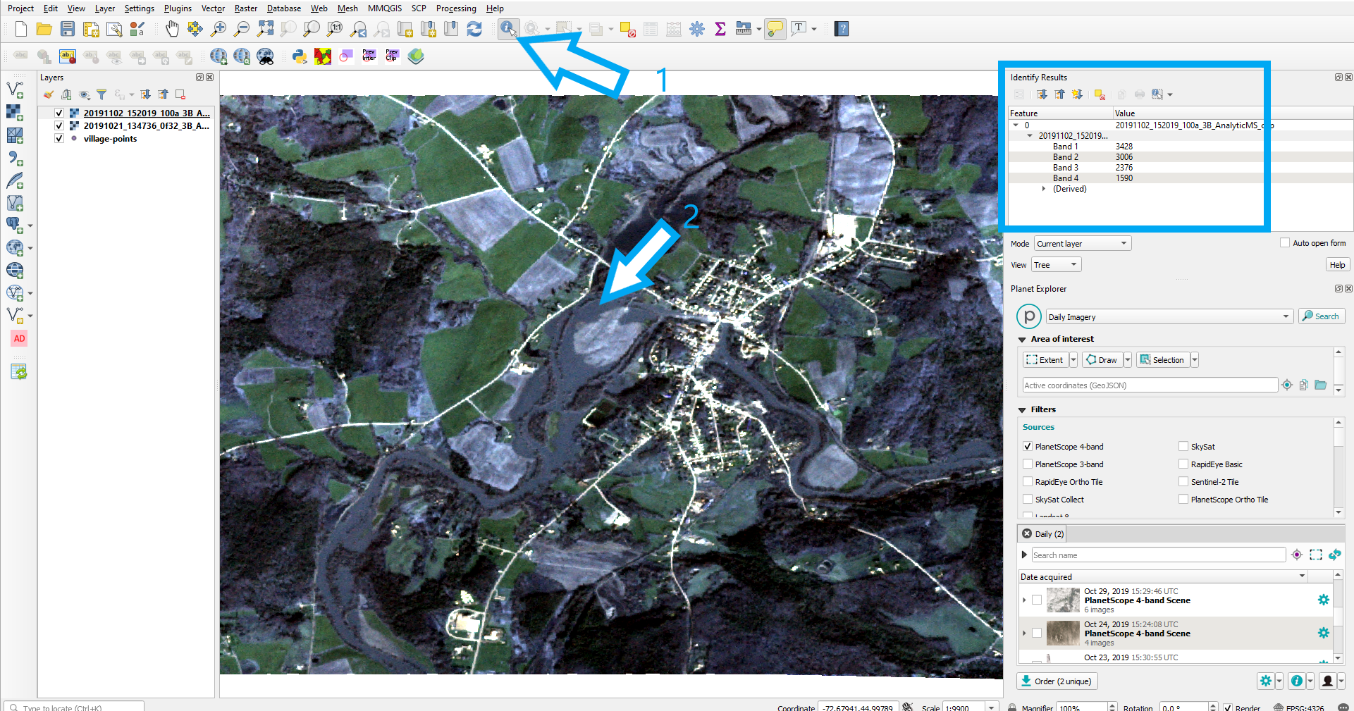
Each of these files has 4 bands. You can see that each pixel contains four values by using the Identify Features button to view some of these values. PlanetScope bands are ordered: blue, green, red, NIR. Remember that for the Identify Features tool to work you must have one of the layers selected in the Layers panel (or you can right-click on the map and choose the layer you are identifying).

We want to depict the extent of change in water between the two scenes using a Normalized Difference Water Index (NDWI), which is calculated with Band 2 (corresponding to green) and Band 4 (corresponding to the near-infrared). The formula for NWDI is:

    NDWI = (Green - near infrared) / (Green + near infrared)

In terms of the PlanetScope 4-band imagery, this formula can be expressed as:

    NDWI = (Band 2 - Band 4) / (Band 2 + Band 4)

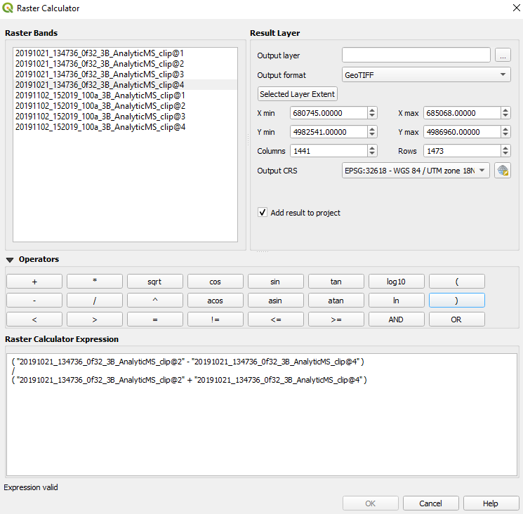
(There are two methods of calculating NDWI, in this tutorial we are using the Green and NIR band method rather than the near infrared and short-wave infrared method.) We want to calculate the NDWI for each of our two images. In QGIS, Click Raster in the menu bar and choose Raster Calculator... All the raster bands will be displayed in the Raster Bands section. Using the formula, double-click the appropriate bands and fill in the appropriate math symbols for the October 21 scene until you have an expression that looks like this. Remember you can double click the raster bands in the Raster Bands list to populate the Raster Calculator Expression input box:

But don’t press OK yet! Here’s the tricky part: these PlanetScope scene values are radiance values and we need what’s referred to as reflectance values. To do this, we have to multiply our data by a certain coefficient that we’ll find in the metadata that came with the datasets we downloaded. Go back to the metadata xml file that came with the October 21 dataset and open it in a text editor (on Windows you would right-click and choose Open with > Notepad) and scroll to the bottom of the file. This is where the coefficients for the scene will be listed. Here is a screenshot of how this looks along with the appropriate coefficients to use. Notice the coefficients we want are listed in the band number 2 and band number 4 sections, respectively.

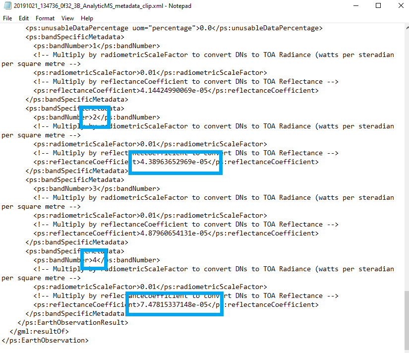
The two coefficients for this image are:

    Band 2: 0.0000438963652969 Band 4: 0.0000747815337148

Applying these multipliers to the bands in the calculation we will have the following expression, which is formatted so you can simply copy/paste if you’d like. (Note that in some cases a copy/paste will cause the Rster calculator to appear strangely formatted but rest assured that the paste did work and the calculation will also still work.) Essentially, you will be replacing the calculation that you placed in the calulator earlier with this one, since it has the coefficients we need.

    (  ( "20191021_134736_0f32_3B_AnalyticMS_clip@2" * 0.0000438963652969 ) ( "20191021_134736_0f32_3B_AnalyticMS_clip@4" * 0.0000747815337148 ) ) /  ( ( "20191021_134736_0f32_3B_AnalyticMS_clip@2" * 0.0000438963652969 )  + ( "20191021_134736_0f32_3B_AnalyticMS_clip@4" * 0.0000747815337148 )  )

Be sure to provide a name for the output in the Output layer input box at the upper-right of the Raster Calculator dialog. A suggestion is to make sure the name has the date of this scene in it. Then click OK. It will do this math on every pixel in the image.

Do this entire process for the November 2 scene, remembering to get the coefficients from its metadata file, as they will be different.

When finished it will look something like this, remembering that your result numbers will be slightly different because your AOI will be slightly different.

McFeeters (1996) reports that the NDWI results in negative or zero pixel values when they represent soil and vegetation but that the results will have positive values when they represent water. In our case, on visual inspection, the data may seem to lend itself to a slightly lower threshold of perhaps -0.1 and higher. To comport with the existing literature and to proceed with the least error of commission, we will still use zero as our lower threshold even though some water may not be captured.

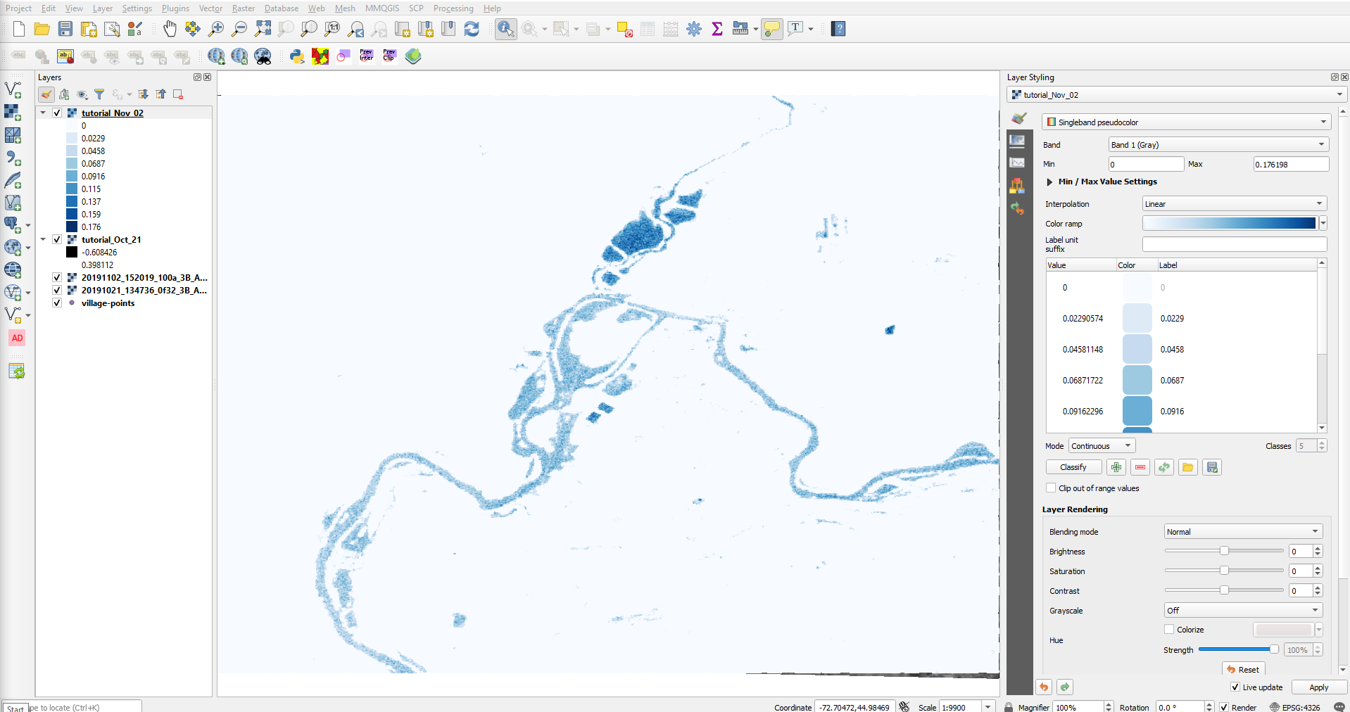
So we are interested in visualizing just the values in both result layers that are greater than zero. Open the Layer Styling Panel if it is not already open using the View drop-down in QGIS’s menu bar, and then Panels > Layer Styling. For both layers, follow the same procedure. In the Layer Styling Panel change the first drop-down to one of the layers that was just calculated (this will probably already be the case), then change the second drop-down to Singleband pseudocolor. Change the Min input box to 0. The Color ramp should be set to Blues if it isn’t already. The project should look something like this:

Double-click the color rectangle next to the “0” value in the Layer Styling Panel, change the Opacity input box to 0% and press OK. This makes all the zero values transparent. Take a look at the result on top of the corresponding scene layer.

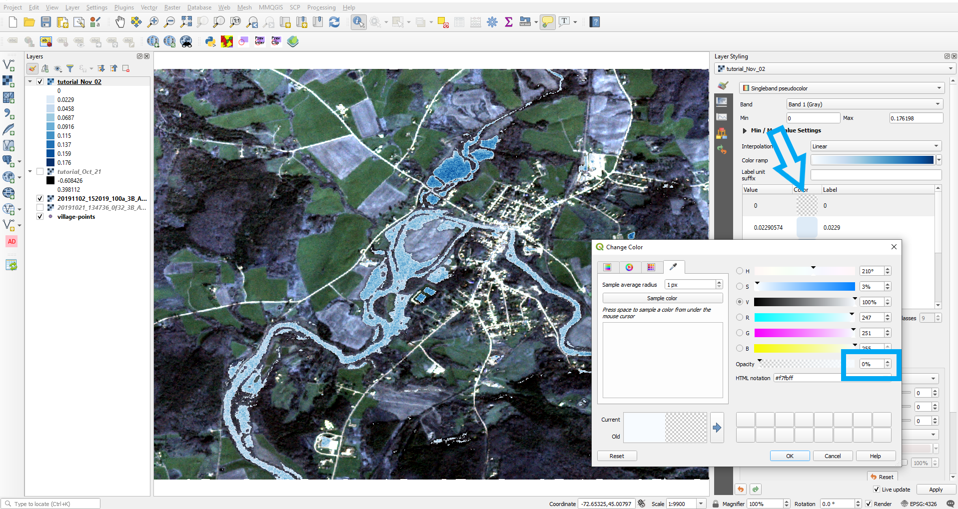
This seems to give us an adequate and conservative approximation of water volume for this scene for our demonstration purposes. Do the same to the other layer. Now we have measurable depictions of the change in water from before a storm event to after a storm event.

Please note, in many cases flood events correspond with high cloud events. Therefore, it may not be possible to perform this same type of analysis on every flood event. Additionally, this analysis is not ground-truthed and no estimate of error was attempted. This tutorial is for demonstration purposes only and fitness for use of this calculation must be made before applying to real-world scenarios.

---

Rate this guide: