In this guide, you'll learn about Planet's automatic detection of pixels which are cloudy or otherwise obscured, so that you can make more intelligent choices about whether the data meets your needs.
In 2018, Planet undertook a project to improve cloud detection, and this guide will focus on the improved metadata that can be used for filtering and the new udm2 asset that provides access to detail classification of every pixel. Planet is not currently planning on removing old cloud cover metadata or the old udm asset.
Finding clear imagery
One of the benefits of accurate and automated cloud detection is that it allows users to filter out images that don't meet a certain quality threshold. Planet's Data API allows users to search based on the value of the imagery metadata.
For example, if you are using the Planet command-line tool, you can search for all four-band PlanetScope scenes that have less than 10% cloud cover in them with the following:
planet data search --item-type PSScene --range cloud_percent lt 10
Planet's cloud detection algorithm classifies every pixel into one of six different categories, each of which has a corresponding metadata field that reflects the percentage of data that falls into the category.
| Class | Metadata field |
|---|---|
| clear | clear_percent |
| snow | snow_ice_percent |
| shadow | shadow_percent |
| light haze | light_haze_percent |
| heavy haze | heavy_haze_percent |
| cloud | cloud_percent |
These can be combined to refine search results even further. An example of searching for imagery that has less than 10% clouds and less than 10% heavy haze:
planet data search --item-type PSScene --range cloud_percent lt 10 --range heavy_haze_percent lt 10
Every pixel will be classified into only one of the categories above; a pixel may be snowy or obscured by a shadow but it can not be both at the same time!
The following example will show how to do a search for imagery that is at least 90% clear using Planet's Python client.
from planet import api
client = api.ClientV1()
# build a filter for the AOI
filter = api.filters.range_filter("clear_percent", gte=90)

# show the structure of the filter
print(filter)
# we are requesting PlanetScope 4 Band imagery
item_types = ['PSScene']
request = api.filters.build_search_request(filter, item_types)

# this will cause an exception if there are any API related errors
results = client.quick_search(request)
# print out the ID of the most recent 10 images that matched
for item in results.items_iter(10):
    print('%s' % item['id'])
The udm2 asset
In addition to metadata for filtering, the udm2 asset provides a pixel-by-pixel map that identifies the classification of each pixel.
In the example below, cloudy pixels are highlighted in yellow, shadows in red and light haze in blue.
| Original image | udm2 overlay |
|---|---|
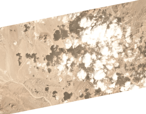 |
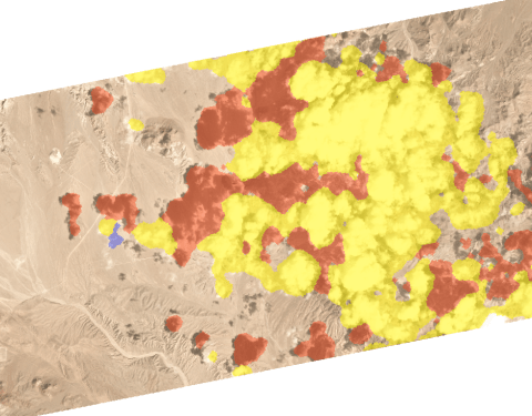 |
20190228_172942_0f1a_3B_Visual.tif |
20190228_172942_0f1a_udm2.tif |
The udm2 structure is to use a separate band for each classification type. Band 2, for example, indicates that a pixel is snowy when its value is 1, band 3 indicates shadow and so on.
The following Python will download the data above and then display pixels that fall into a certain classifications.
item_type = "PSScene"
item_id = "20190228_172942_0f1a"
import time

# activate assets
assets = client.get_assets_by_id("PSScene", item_id).get()
client.activate(assets["analytic"])
client.activate(assets["udm2"])

# wait until activation completes
while True:
    assets = client.get_assets_by_id("PSScene", item_id).get()
    if assets["analytic"].has_key("location") and assets["udm2"].has_key("location"):
            break
    time.sleep(10)
# start downloads
r1 = client.download(assets["analytic"], callback=api.write_to_file())
r2 = client.download(assets["udm2"], callback=api.write_to_file())
# wait until downloads complete
r1.wait()
r2.wait()
img_file = r1.get_body().name
udm_file = r2.get_body().name
print("image: {}".format(img_file))
print("udm2:  {}".format(udm_file))
import rasterio
from rasterio.plot import show
with rasterio.open(udm_file) as src:
    shadow_mask = src.read(3).astype(bool)
    cloud_mask = src.read(6).astype(bool)
show(shadow_mask, title="shadow", cmap="binary")
show(cloud_mask, title="cloud", cmap="binary")


mask = shadow_mask + cloud_mask
show(mask, title="mask", cmap="binary")

with rasterio.open(img_file) as src:
    profile = src.profile
    img_data = src.read([3, 2, 1], masked=True) / 10000.0 # apply RGB ordering and scale down
show(img_data, title=item_id)

img_data.mask = mask
img_data = img_data.filled(fill_value=0)
show(img_data, title="masked image")

The image stored in img_data now has cloudy pixels masked out and can be saved or used for analysis.