Time to complete: this tutorial is expected to take anywhere from 30 minutes to 2 hours depending on your ArcGIS Pro and satellite imagery familiarity.
IT'S INSTALL TIME
First things first, you will need to purchase a Planet subscription here. The Planet Explorer ArcGIS Pro Add-In can be installed, but not used, until you log in. Second, if you don't already have ArcGIS Pro you will need to purchase, install, and log in to it.
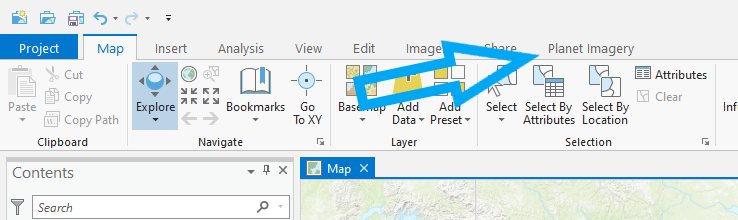
If ArcGIS Pro is open, it is best to close it before installing the Add-In. You can download the Add-In here. Once downloaded, double-click the Add-In file to validate it and install it. Click Install Add-In. Now open ArcGIS Pro and verify that the Add-In was installed correctly by clicking on the Project tab from a new open project, then clicking Add-In Manager from the list at left. If the Add-In is installed it will be listed in the My Add-Ins section. Click the back arrow to go back to the new project. Notice that a new ribbon is added and accessed by clicking on the Planet Imagery tab.
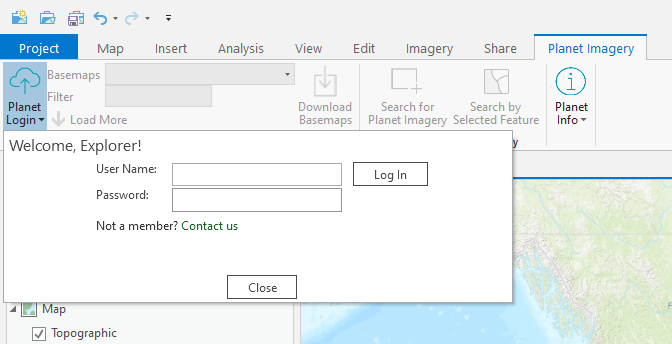
On the ribbon, click Planet Login to fill in the credentials you obtained earlier when you purchased a Planet subscription. Click log in once you have filled in your credentials. Note that login credentials must be re-entered with each new ArcGIS Pro session. The Planet ribbon (i.e., the new set of buttons now available near the top of the ArcGIS Pro window) is now active.
The Basemaps drop down menu contains several mosaics to browse. Click on one and notice how it is now placed in the left-hand Contents pane under the heading Planet Basemaps, where you can turn it on and off or remove it. Use the Load More button to load more mosaics into the drop-down. Some of the mosaics have partial coverage, some have snow. They are interesting to take a look through.
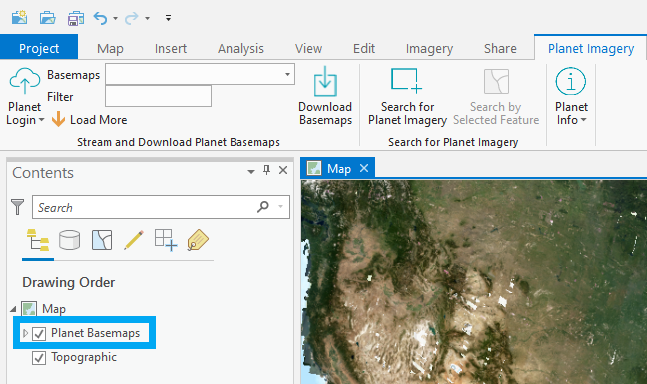
Remove the mosaic(s) once you are finished browsing them to keep the project clean by right-clicking on the Planet Basemaps heading and choosing Remove.
IT'S CRAZY QUICK TIME
Sometimes people want to jump right in. If that sounds like you, use this section as your 30-second quick-start and then proceed to the tutorial. Otherwise, skip to the tutorial.
- Zoom to an interesting location
- Click Planet Imagery > Search for Planet Imagery
- Draw a rectangle around your area of interest and click Search in the Search For Planet Imagery panel
- Browse the results and click Order
IT'S TUTORIAL TIME
Flooding occurred along the Missisquoi River, Vermont in early November 2019. Let’s take a look at what happened there by exploring a location that was affected: Richford, Vermont. We’ll see what satellite imagery is available before and during the flood, which took place on and around November 1, 2019. We’ve extracted the village point for Richford from OpenStreetMap and put it in a feature service, located in this directory. Download that file and its other components (i.e., also download the .cpg, .dbf, .prj, .qpj, .shx files) then drag and drop the file with the .shp extension onto the ArcGIS Pro Contents pane. Make sure it is at the top of the Drawing Order and use Alt + layer-click several times or use the mouse wheel to zoom all the way to the point. It is helpful to have the default ArcGIS Pro basemap on to locate the general town boundaries.
Click Search for Planet Imagery in the Planet Imagery ribbon. A toolbar pops up on the bottom of the map view.
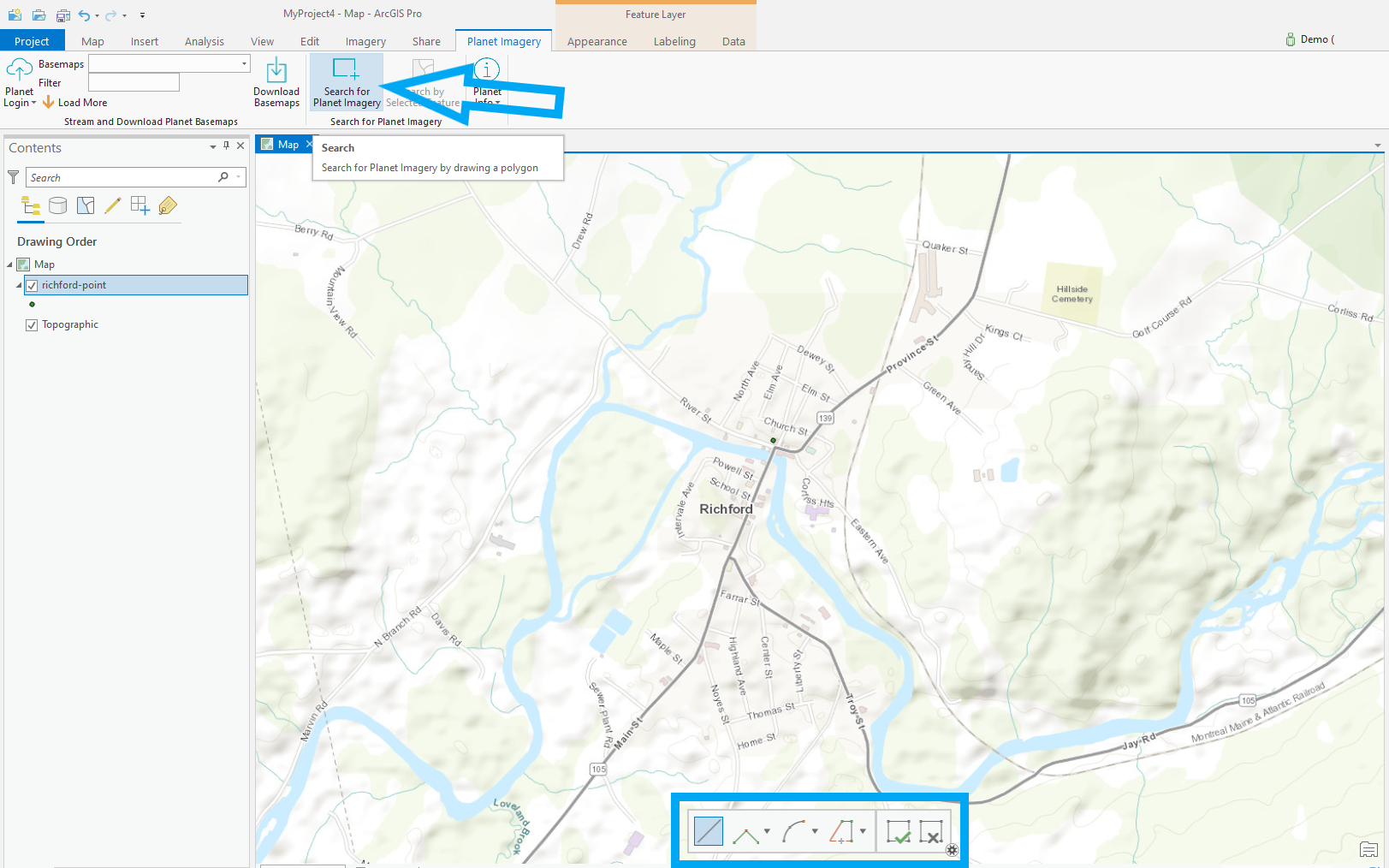
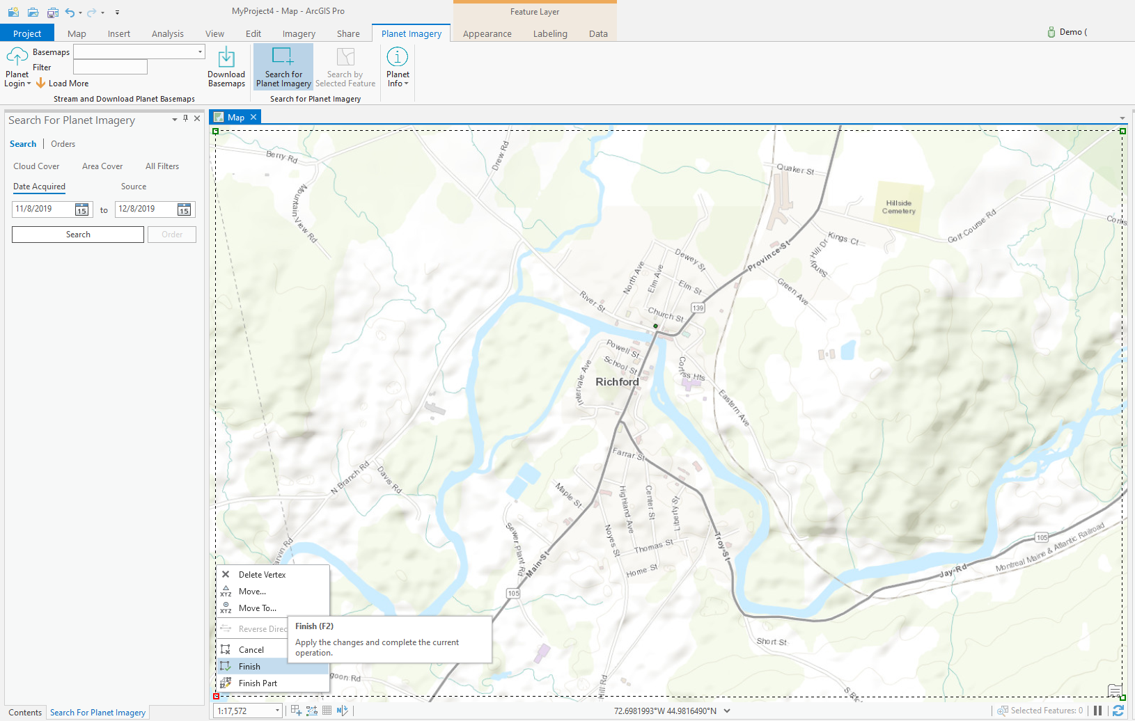
Using the tool that is already selected, the Line tool, click on the map view to form a square around this location. At the last point of the square, right-click and choose Finish. This indicates the search area, also called Area of Interest (AOI), that will be used for your imagery searches. Your AOI will not exactly match those in the tutorial. Did you make a mistake and want to try again? Just start a new AOI. When it is completed, the old one will be discarded. But for this tutorial an approximation is okay. Notice that a new pane, and pane tab, at the left-hand side of the ArcGIS Pro window will appear that is titled Search For Planet Imagery.
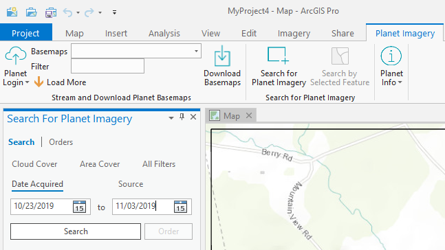
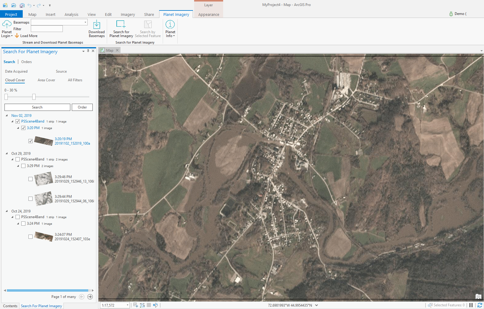
If you need to return to the Contents pane at any time, click the tab labeled Contents at the bottom-left of the ArcGIS Pro window or go to View > Contents in the ribbon. Next, because we want imagery from a specific time period, use the Date Acquired input boxes in the Search For Planet Imagery pane to provide two dates: 10/23/2019 and 11/03/2019. These are found in the Search section of the pane.
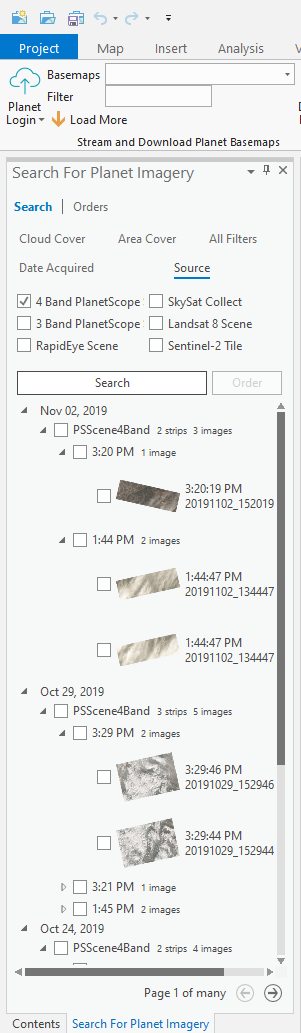
Click the Source tab and ensure that just 4 Band PlanetScope imagery is selected. Click Search. A few PlanetScope 4-band Scenes now appear under the Search button. Unfold these using the down-arrows and browse the images in the map view by clicking them on and off here. The small preview next to each scene will indicate the general amount of cloud cover in the scene. While your list of available scenes may look different depending on the size of the rectangle you drew, in our case some of the scenes in our list look cloudy.
Click the Cloud Cover tab, then move the upper slider down to 30%, then press Search. Unfold these results and notice that fewer images are available now that we've constrained the cloud cover parameters.
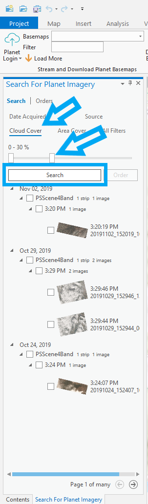
The Nov 02, 2019 image shows some of the flooding that occurred during this "Halloween" storm. It will be perfect for our analysis.
The other images aren't good enough for the analysis. To gain an understanding of the typical amount of water here during a non-storm-event, it will be okay to extend the date search to 10/21/2019 for the earlier date and to keep 11/03/2019 for the later date. Make that change in the Date Acquired tab and click Search again. Browsing through the new Oct 21, 2019 images, notice that the image with the suffix "_0f32" will be perfect for the pre-flood part of the analysis.
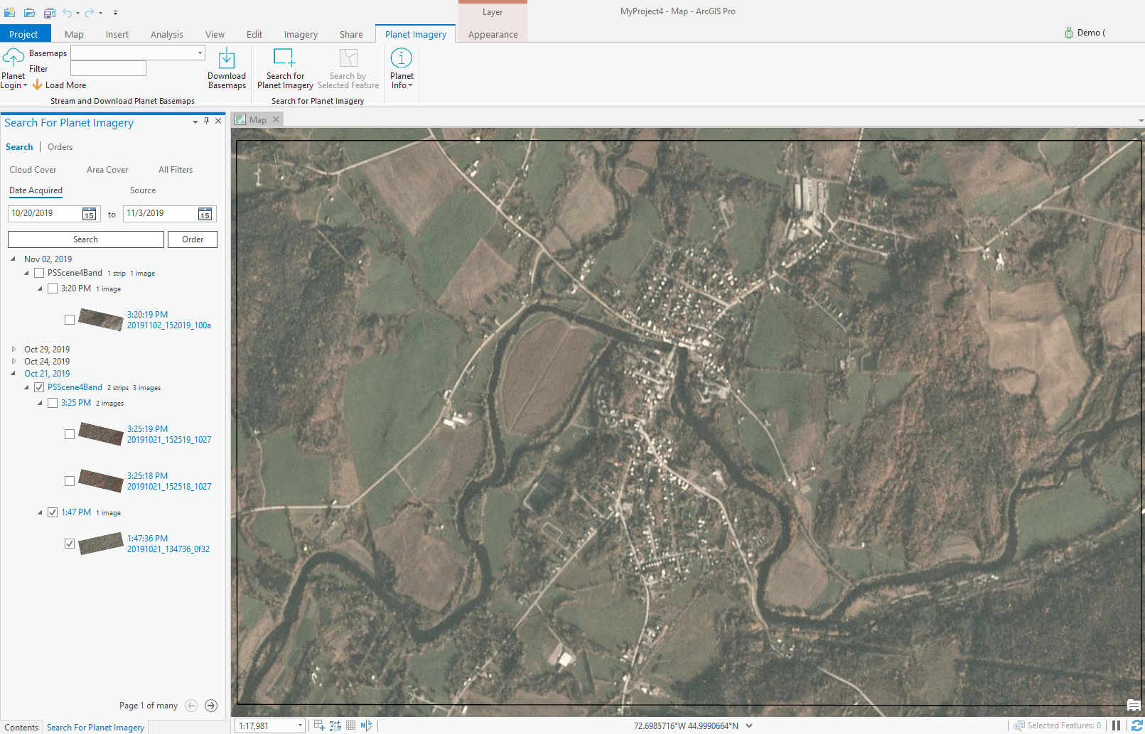
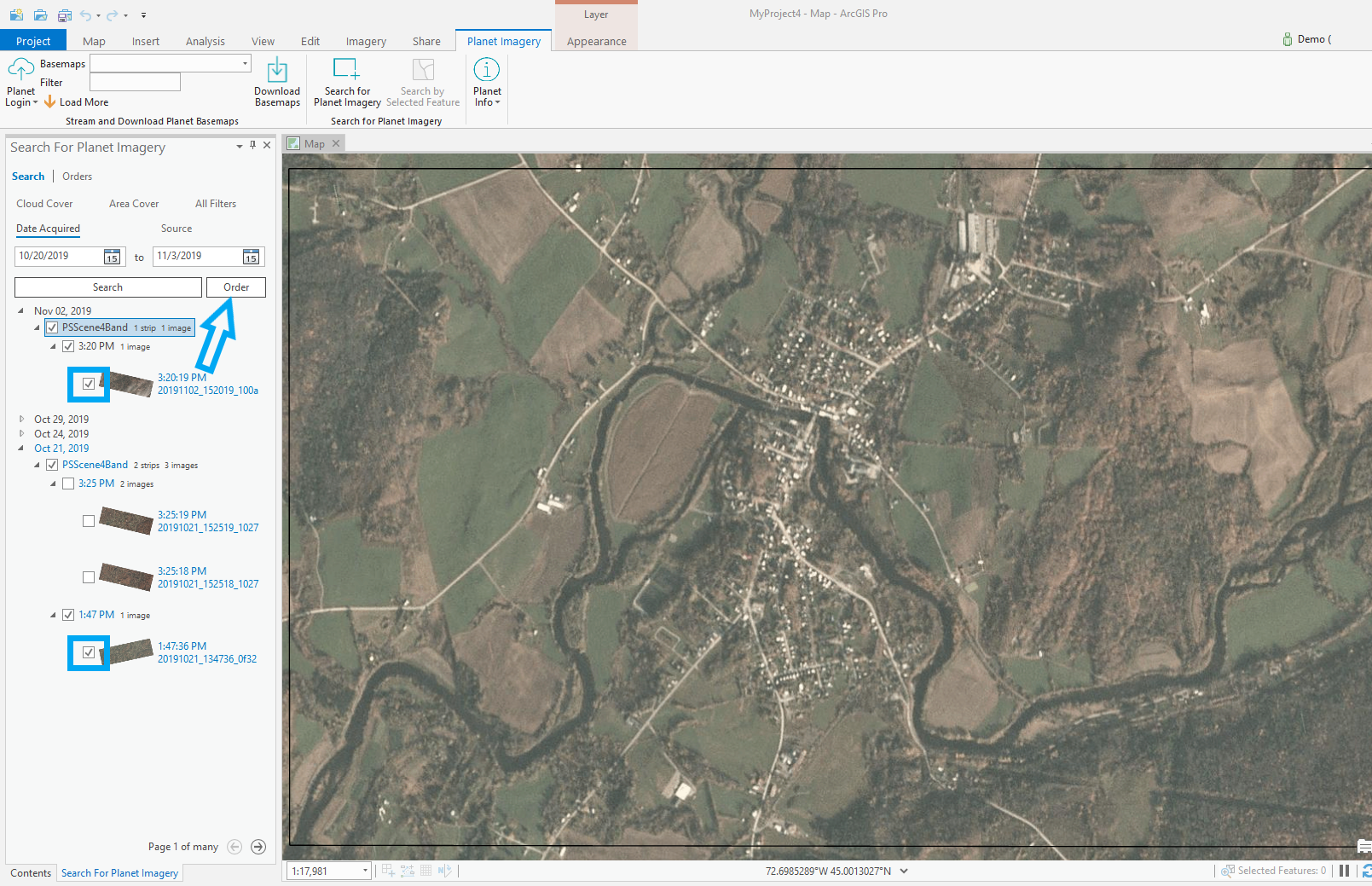
It's now time to place an order to get the imagery since previously we were just looking at previews. The two scenes that we want to order are the Nov 02, 2019 scene with the "_100a" suffix and the Oct 21, 2019 scene with the "_0f32" suffix. Make sure these are clicked on and then click the Order button.
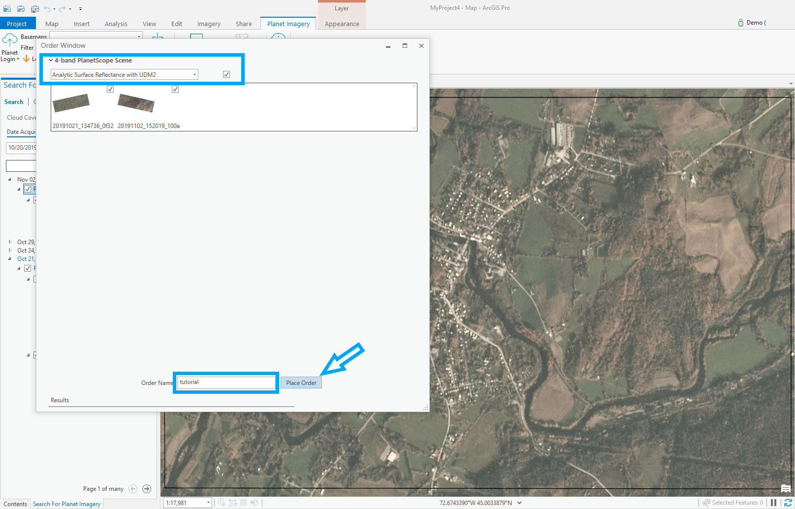
The Order Window pops up. Unfold the 4-band PlanetScope Scene listing at the top, choose Analytic Surface Reflectance with UDM2 in the drop-down, and click the Select All box next to it to select both images that we had selected in the main Search For Planet Imagery pane. In the Order Name: box type in a name for the order and then click Place Order.
A results bar appears at the bottom of the Order Window.
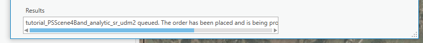
Click the Orders tab in the main Search For Planet Imagery pane. This is where the order will appear once it is ready. Click the Refresh button to check if it is. The Status for your order will show "running" while it is processing and "success" when it is finished processing and ready to download. Once it is finished, scroll the bar to the right if needed and click the Download link. You are prompted for a download location. Click OK once you select a location for the scenes. A notification lets you know when the download is complete.
Using Windows Explorer, navigate to the location where you downloaded the files and click through the various folders until you see the two .tif files we need (they will be in separate folders but it is good to verify they are both there, while leaving them in their original folders):
20191021_134736_0f32_3B_AnalyticMS_SR.tif
20191102_152019_100a_3B_AnalyticMS_SR.tif
Add them to ArcGIS Pro by dragging and dropping the tif files--you know which one you need by looking at the Size in Windows Explorer, the largest ones in each folder are the correct ones--onto the ArcGIS Pro Contents pane. Click the Planet Daily Imagery box off or remove it to keep the ArcGIS Pro project clean.
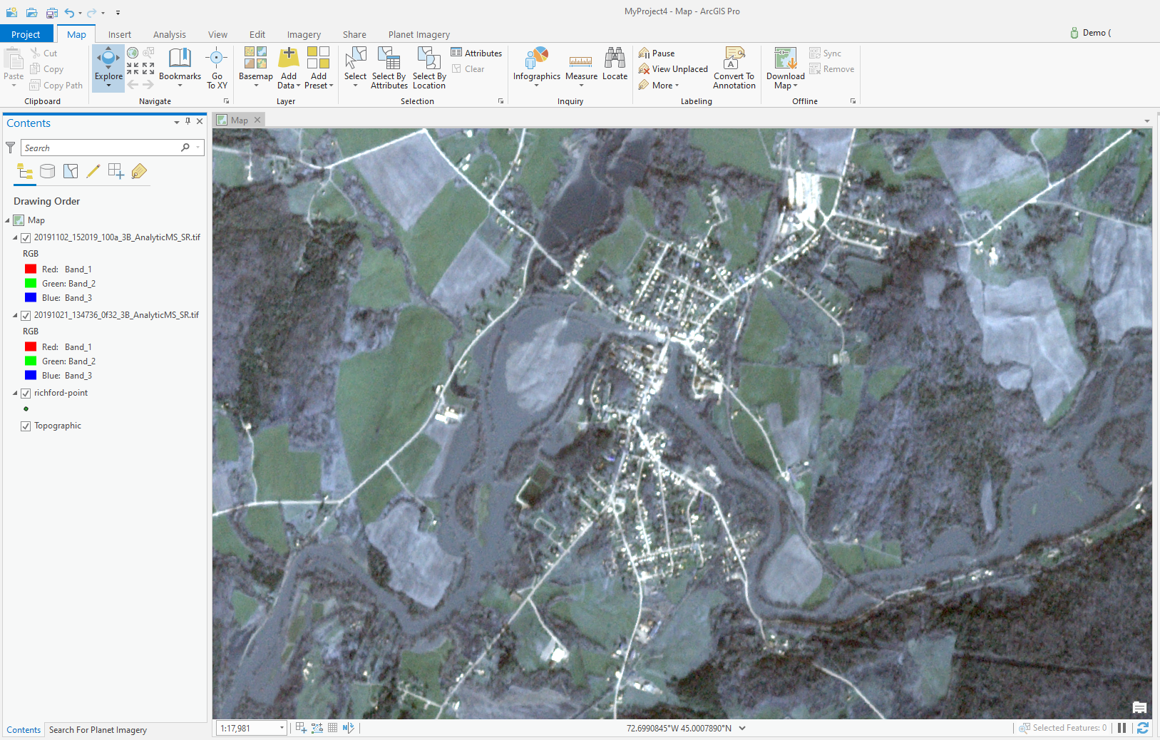
Notice that the first one in the above screenshot is the November 2 dated scene, which is apparent from the beginning of the file name, and the second is the October 21 dated scene. These files each have 4 bands despite the fact that ArcGIS Pro has displayed only three of them automatically. You can verify that each pixel contains four values, one for each band, by looking at the symbology for one of the scenes. Do this by right-clicking a scene in the Contents pane, choosing Symbology and clicking the drop-down next to Red in the Symbology pane that appears at the right-hand side of the ArcGIS Pro window. There will be 4 bands to choose from in this drop-down. Leave it as is, however.
We want to depict the extent of change in water between the two scenes using a Normalized Difference Water Index (NDWI), which is calculated with Band 2 (corresponding to green) and Band 4 (corresponding to the near-infrared). The formula for NWDI is:
NDWI = (Green - near infrared) / (Green + near infrared)
In terms of the PlanetScope 4-band imagery, this formula can be expressed as:
NDWI = (Band 2 - Band 4) / (Band 2 + Band 4)
(There are two methods of calculating NDWI, in this tutorial we are using the Green and NIR band method rather than the near infrared and short-wave infrared method.) We want to calculate the NDWI for each of our two images. ArcGIS Pro has several pre-configured indices computations listed in the Imagery ribbon under Indices. However, our NDWI index will need to be computed via the raster calculator. Please note that this tool is only available with either the Spatial Analyst license or the Image Analyst license.
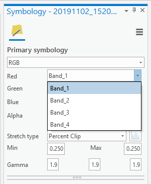
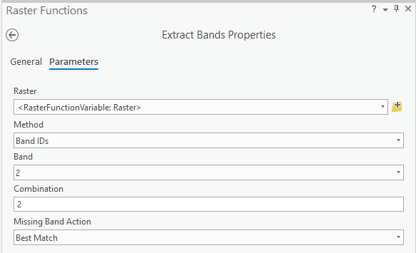
Before we use the raster calculator, we first need to extract the bands from the images. To do this, open Raster Functions in the Imagery pane.
In the raster Functions pane, go to Data Management > Extract Bands. Use the drop-down to choose the Oct 21 tif file. Make sure the drop-down under Band says "2", and type "2" in the Combination text box (i.e., delete the other numbers in that box). Leave everything else the same and press Create new layer. Re-name this layer by clicking on its name in the layer list, which is the list of datasets in the Contents pane, and typing, "Oct 21 Band 2". Repeat this process for the same Oct 21 tif file except this time for band number 4, renaming it to "Oct 21 Band 4". Repeat the process again two more times for the Nov 02 tif file, first for band number 2 and then again for band number 4.
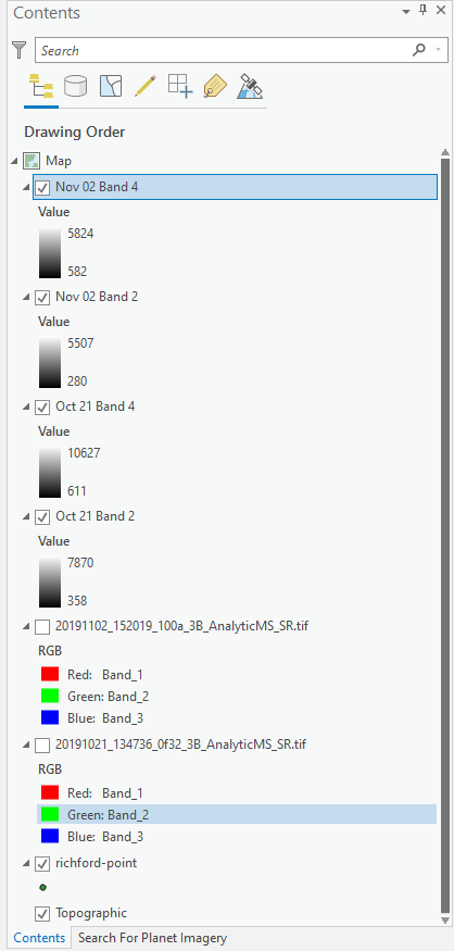
The Contents pane should now look like this:
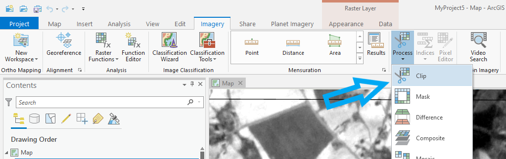
At this point we should also clip the bands to the area of interest. With the Nov 02 Band 4 layer active and selected (this means you need to actually click on the name of the layer so that it is highlighted) in the Contents pane, click Clip. A new layer appears in the Contents pane that is clipped to the map view's extent named "Clip_Nov 02 Band4."
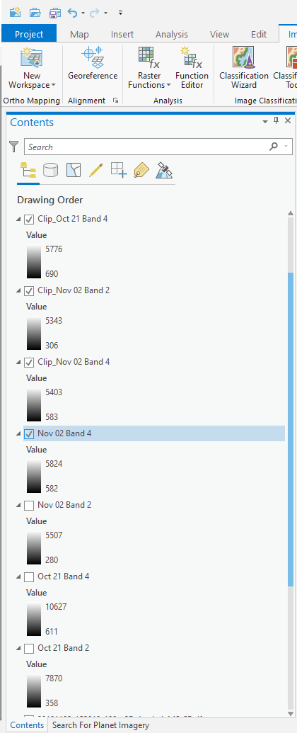
Do this for all 4 band layers so that the Contents pane now looks like this:
Now we're ready for the NDWI calculation. Click Tools in the Analysis ribbon to open the Geoprocessing pane on the right-hand side of the ArcGIS Pro window. Type
raster calculator
in the Find Tools box and select it in the list that appears. Note that it will appear in the list twice if you have both the Image Analyst license and the Spatial Analyst license. Either one is fine.) Expand the raster calculator panel so you can see your work better. All the rasters in the map will be displayed in the Rasters section. Using the NDWI formula, double-click the appropriate bands and fill in the appropriate math symbols for the October 21 scene until you have an expression that looks like what we show below. Note that we've named the result "Oct21NDWI." Remember you can double click the raster layers in the Rasters list to populate the expression input box:
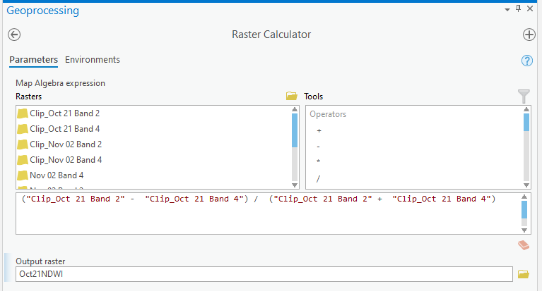
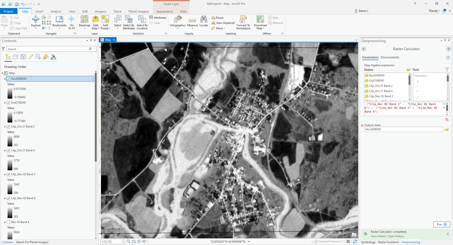
Click Run in the lower right-hand corner of the Geoprocessing panel. The computed layer will appear in the Contents pane. Do the same thing for the Nov 02 computation. The results will look something like what we show below, though your raster min and max values will vary depending on your exact area of interest.
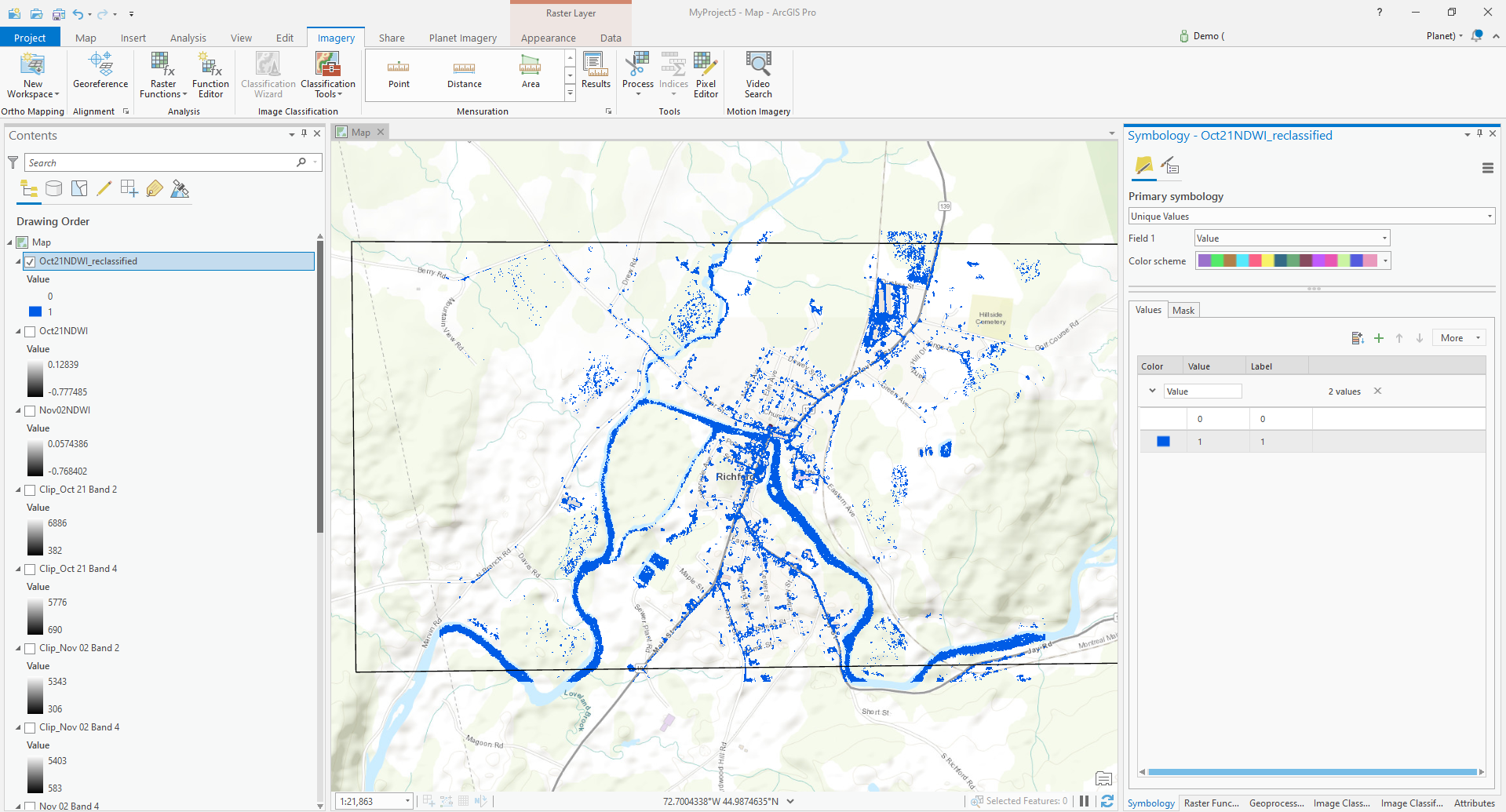
To better visualize the results, we'll reclassify the data using a "Con" expression in the Raster calculator. Go back to the Raster Calculator in the Geoprocessing tab as before and type the following expression to create a new output raster that assigns a 1 pixel value to all pixels between two values in the result data and a 0 to all other values. Note the use of our output result name in the expression. Make sure whatever you named your output result is put into the calculation if you've named yours differently. Name this output raster "Oct21NDWI_reclassified".
Con(( "Oct21NDWI">-0.35) & ("Oct21NDWI"<-0.2),1,0)
In the Symbology tab for this new layer, choose Unique Values, change the 0 value color to No Color and the 1 value color to a blue hue as shown:
Do the same thing for the Nov02NDWI layer using the following expression:
Con(( "Nov02NDWI">-0.26) & ("Nov02NDWI"<-0.1),1,0)
Now we can see the difference between the pre-storm event and the storm event:
Please note: A land-water threshold was manually applied to classify the images into two classes, land and water. These were -0.35 and -0.2 for the October 21 results and -0.26 and -0.1 for the November 02 results. These suitable land-water thresholds for each index were determined through trial and error and comparison to reference maps generated using visual interpretation. For visual interpretation of water bodies, the near-infrared (NIR) band is usually preferred, because NIR is strongly absorbed by water and is strongly reflected by the terrestrial vegetation and dry soil - source.
Rate this guide: