Overview
The purpose of this tutorial is to use Planet imagery to calculate an approximate percentage change in reservoir water levels.
How To Get Started
Before we start our analysis we need to ensure we have the required packages and Planet satellite images.
Requirements
Software & Python Libraries
You will need:
- Python 3
- GDAL
- scipy & numpy
- skimage
- requests
- OpenCV
- imutils
- The Planet CLI (optional)
- Your Planet API Key
How to Export Planet API Key and Install Packages
To export your Planet API Key to your environment:
export PLANET_API_KEY=a3a64774d30c4749826b6be445489d3b # (not a real key)
You can find GDAL installation instructions here. For installation of scipy & numpy, see this page.
To install the Python libraries, do:
$ python -m pip install requests
$ python -m pip install opencv-python
$ python -m pip install scikit-image
$ python -m pip install imutils

# optionally:
$ python -m pip install planet
Once installation is complete, you're ready to start with Step 1 below.
A note about Planet Imagery Product Compatability: this tutorial is compatable with all ItemTypes & Asset Types.
Download Images at Two Time Points
First, let's download images of the same Reservoir in California, 2 weeks apart.
You can use the Data API to search for, activate & download these images, or optionally you can use the planet CLI.
How to Download Images with Planet CLI
To use the CLI, do:
$ planet data download --item-type REOrthoTile --asset-type visual --string-in id 20160707_195146_1057917_RapidEye-1
$ planet data download --item-type REOrthoTile --asset-type visual --string-in id 20160722_194930_1057917_RapidEye-2
You now have the two Planet 'visual' GeoTIFF format images in your current directory.
N.B.: As this is just an example, we are using Planet's 'visual' asset type. If we wanted a more accurate measurement we would use the higher bit-depth 'analytic' product.
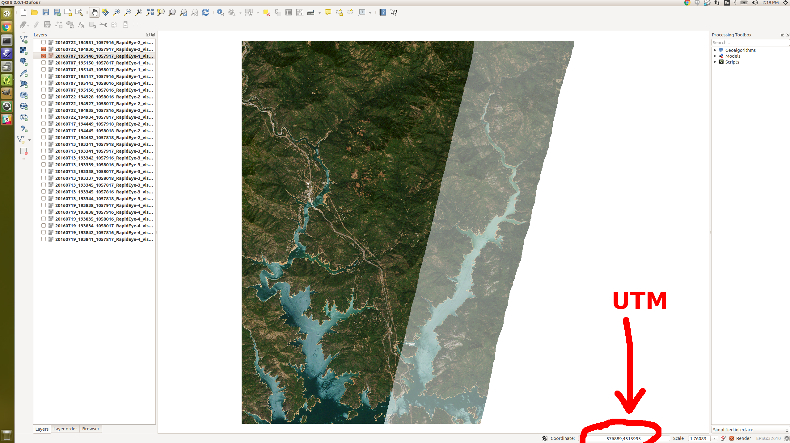
Use QGIS to Select Common Window to Compare
Our scenes don't overlap perfectly, and for the calculation to be accurate we'd prefer they did. The GDAL Warp command enables us to do this crop.
With QGIS we can find the overlapping rectangle between the two scenes. Move your mouse to where you estimate the corners might be, and take note of the numbers from the 'coordinates' box on the bottom menu bar.
Crop Images With GDAL Warp Command
We then run the following bash commands:
gdalwarp -te 547500 4511500 556702 4527000 1057917_2016-07-07_RE1_3A_Visual.tif 20160707.tif
gdalwarp -te 547500 4511500 556702 4527000 1057917_2016-07-22_RE2_3A_Visual.tif 20160722.tif
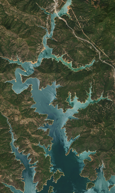
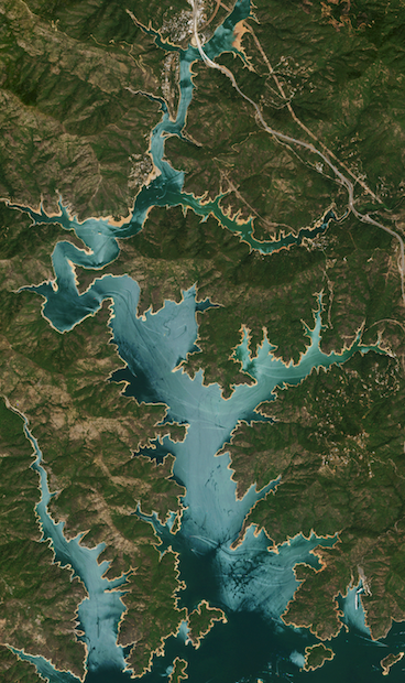
Find the Water
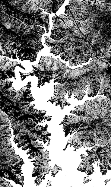
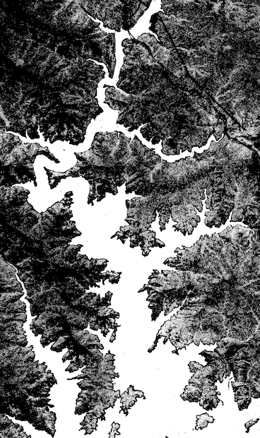
In order to find the water we want to extract the blue hues within the image. Using OpenCV, we convert the BGR colorspace to HSV and create a threshold to extract the blue water. As you can see below, the mask we created differentiates the water from the land.
Create a Mask Using Threshold
import cv2 as cv

a = cv.imread('20160707.tif')
b = cv.imread('20160722.tif')

hsv_a = cv.cvtColor(a, cv.COLOR_BGR2HSV)
hsv_b = cv.cvtColor(b, cv.COLOR_BGR2HSV)

low = np.array([55, 0, 0])
high = np.array([118, 255, 255])

inner_a = cv.inRange(hsv_a, low, high)
inner_b = cv.inRange(hsv_b, low, high

cv.imwrite('inner_a.png', inner_a)
cv.imwrite('inner_b.png', inner_b)
Mask A
Mask B
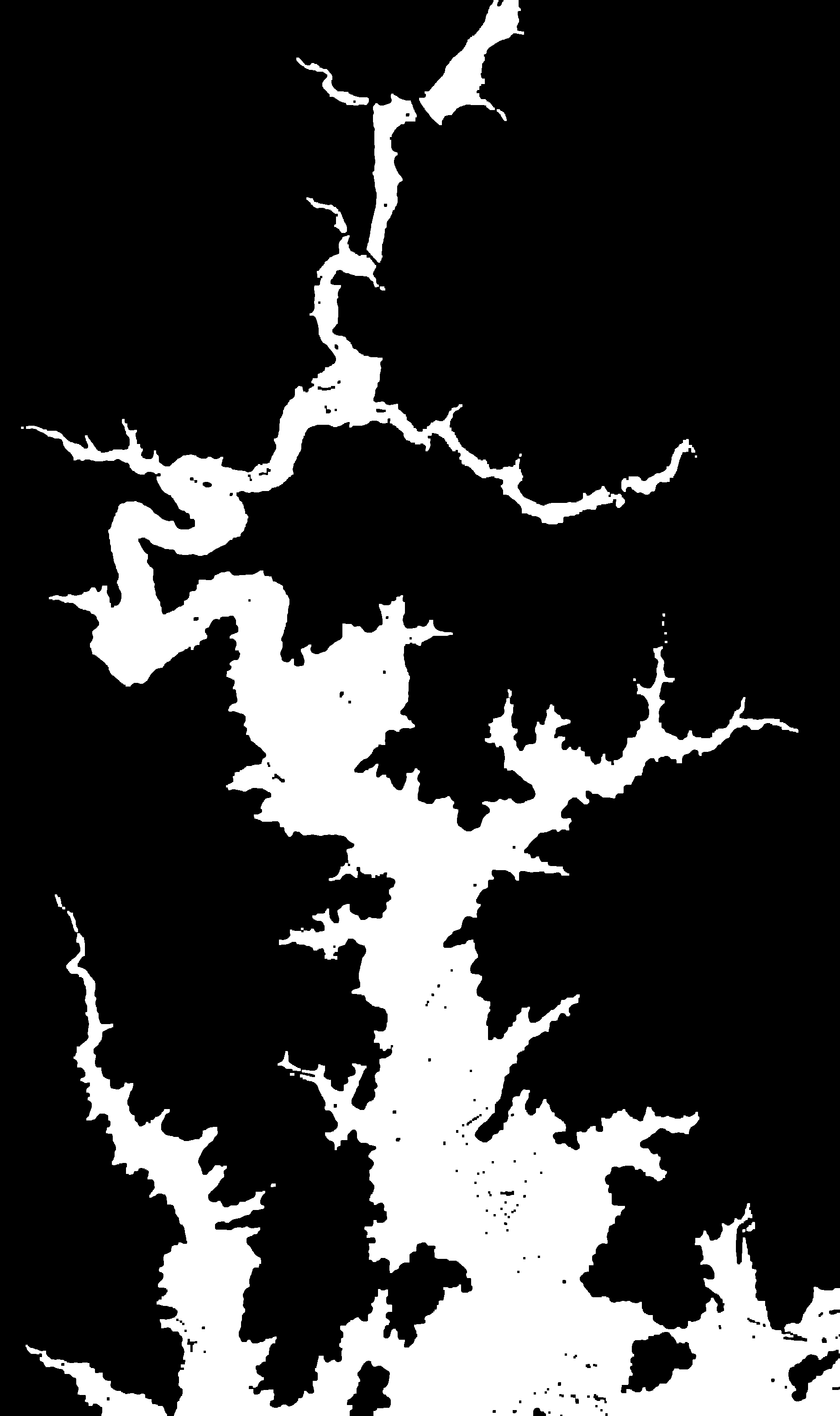
Cleaning up the Mask Using Erosion and Dilation
We currently have some noise in our mask that we can eliminate using two morphological operations, erosion and dilation. The purpose of these operations to ensure we have a clear separation between the background and foreground, or land and water.
kernel = np.ones((5,5),np.uint8)

erosion_a = cv.erode(inner_a,kernel,iterations = 2)
erosion_b = cv.erode(inner_b,kernel,iterations = 2)

innerA = cv.dilate(erosion_a,kernel,iterations = 1)
innerB = cv.dilate(erosion_b,kernel,iterations = 1)

cv.imwrite('innerA.png', innerA)
cv.imwrite('innerB.png', innerB)
Mask A

Mask B
Watershed Algorithm
In order to calculate the changes in water levels we need to know the area of the water in the image. We will use a segmentation technique so we only focus on the water and ignore everything else. The watershed algorithm returns a numpy array of labels with unique values corresponding to the pixel value.
from scipy import ndimage
from skimage.feature import peak_local_max
from skimage.segmentation import watershed
import numpy as np

eucl_a = ndimage.distance_transform_edt(innerA)
eucl_b = ndimage.distance_transform_edt(innerB)

localMaxA = peak_local_max(eucl_a, indices=False, labels=innerA)
localMaxB = peak_local_max(eucl_b, indices=False, labels=innerB)

markers_a = ndimage.label(localMaxA, structure=np.ones((3, 3)))[0]
markers_b = ndimage.label(localMaxB, structure=np.ones((3, 3)))[0]

labels_a = watershed(-eucl_a, markers_a, mask=innerA)
labels_b = watershed(-eucl_b, markers_b, mask=innerB)
Calculating Area Using Contours and Overlaying Mask
Once we have our labels, we loop over each unique label and look for the values that correspond with the foreground, or water. After applying those values to our mask, we then grab the contour of each object in our mask in order to perform our calculations on it. By adding the area of each individual contour to the total area, we are able to approximate the area of the water in our image.
Note: I added lines to fill the contours and save the image for visualization purposes but this isn't necessary for our calculation.
Python Function to Find Area
def get_area(labels, inner_mask, img):
    area = 0
    for label in np.unique(labels):

        if label== 0:
            continue

        mask = np.zeros(inner_mask.shape, dtype="uint8")
        mask[labels == label] = 255

        contours = cv.findContours(mask, cv.RETR_EXTERNAL, cv.CHAIN_APPROX_SIMPLE)
        contours = imutils.grab_contours(contours)
        cv.fillPoly(img, pts=contours, color=(0,255,255))

        a = cv.contourArea(contours[0])
        area+=a

    cv.imwrite('mask.png', img)

    return area

area_a = get_area(labels_a, innerA, a)
area_b = get_area(labels_b, innerB, b)
Image A
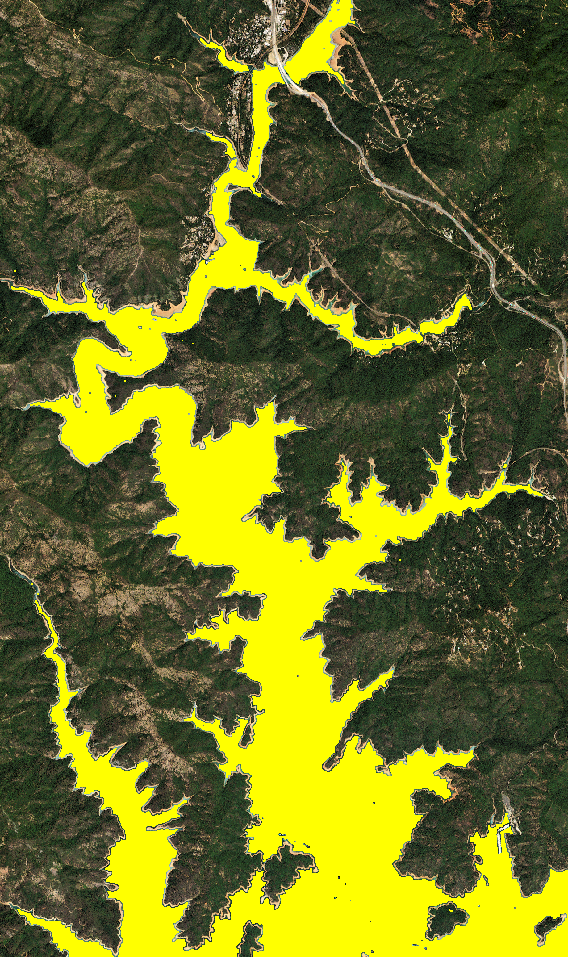
Image B

Apply Function to get Area and Water Change
After we apply our function to both planet images, we now know the approximate change in water reservoir water levels between the times both these images were captured.
area_a = mask_img(labels_a, innerA, a)
area_b = mask_img(labels_b, innerB, b)
water_level_diff = area_b/float(area_a)
Output
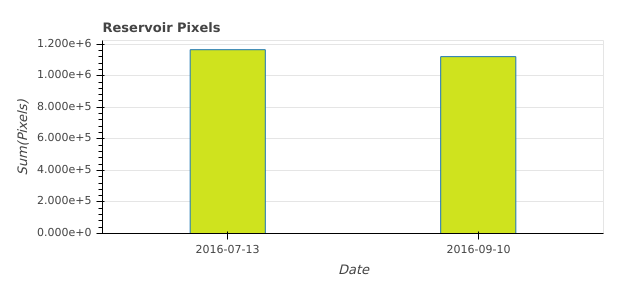
Area A = 1164765.0
Area B = 1120738.5
Water Level Difference = 0.9622013882628685
Percent change = -3.7798611737131504%
Data Visualization Section
Our last step is to plot a bar chart to represent the difference in water levels.
from bokeh.io import output_file, show
from bokeh.plotting import figure
import bokeh.plotting as bk

dates = ['2016-07-13', '2016-09-10']
pixels = [area_a, area_b]

plt = figure(x_range=dates, plot_height=275, title="Reservoir Pixels",
           toolbar_location=None, tools="")

plt.vbar(x=dates, top=pixels, width=0.3, fill_color="#cfe31e")

plt.xgrid.grid_line_color = None
plt.y_range.start = 0
plt.xaxis.axis_label = "Date"
plt.yaxis.axis_label = "Sum(Pixels)"

#saves as a html file
bk.save(plt)
show(plt)
Water Changes
Questions or comments about this guide? Join the conversation at Planet Community.
Rate this guide: